Microsoft Excel is primarily designed to manipulate numbers, so it provides a handful of different ways to perform basic math operations as well as more complex calculations. In our last tutorial, we discussed how to multiply cells in Excel. In this tutorial, we will take a step further and look at how you can quickly multiply entire columns.
How to multiply two columns in Excel
As is the case with all basic math operations, there is more than one way to multiply columns in Excel. Below, we will show you three possible solutions so you can choose the one that works best for you.
How to multiply one column by another with multiplication operator
The easiest way to multiply 2 columns in Excel is by making a simple formula with the multiplication symbol (*). Here's how:
- Multiply two cells in the first row.
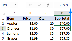
Supposing, your data begins in row 2, with B and C being the columns to be multiplied. The multiplication formula you put in D2 is as plain as this:
=B2*C2 - Double-click the small green square in the lower-right corner of D2 to copy the formula down the column, until the last cell with data. Done!

Since you use relative cell references (without the $ sign) in the formula, the references will change based on a relative position of the row where the formula is copied. For example, the formula in D3 changes to =B3*C3, the formula in D3 becomes =B4*C4, and so on.

How to multiply two columns with PRODUCT function
If you prefer working with Excel functions rather than expressions, you can multiply 2 columns by using the PRODUCT function, which is a specially designed to do multiplication in Excel.
For our sample data set, the formula goes as follows:
=PRODUCT(B2:C2)
As with the multiply symbol, the key point is using relative cell references, so that the formula can adjust properly for each row.
You enter the formula in the first cell, and then copy it down the column as explained in the above example:

How to multiply two columns with an array formula
One more way to multiply entire columns in Excel is by using an array formula. Please don't feel discouraged or intimidated by the words "array formula". This one is very straightforward and easy to use. You simply write down the ranges you want to multiply separated by the multiplication sign, like this:
=B2:B5*C2:C5
To insert this multiplication formula in your worksheets, perform these steps:
- Select the entire range where you want to enter the formula (D2:D5).
- Type the formula in the formula bar, and press Ctrl + Shift + Enter. As soon as you do this, Excel will enclose the formula in {curly braces}, which is an indication of an array formula. In no case should you type the braces manually, that won't work.
As the result, Excel will multiply a value in column B by a value in column C in each row, without you having to copy the formula down.

This approach might be useful if you want to prevent accidental deletion or alteration of the formula in individual cells. When such an attempt is made, Excel will show a warning that you cannot change part of an array.
How to multiply multiple columns in Excel
To multiply more than two columns in Excel, you can use the multiplication formulas similar to the ones discussed above, but include several cells or ranges.
For example, to multiply values in columns B, C and D, use one of the following formulas:
- Multiplication operator:
=A2*B2*C2 - PRODUCT function:
=PRODUCT(A2:C2) - Array formula (Ctrl + Shift + Enter):
=A2:A5*B2:B5*C2:C5
As shown in the screenshot below, the formulas multiply numbers and percentages equally well.

How to multiply a column by a number in Excel
In situations when you want to multiply all values in a column by the same number, proceed in one of the following ways.
Multiply a column by a number with a formula
As it happens, the fastest way to do multiplication in Excel is by using the multiply symbol (*), and this task is no exception. Here's what you do:
- Enter the number to multiply by in some cell, say in B1.
In this example, we are going to multiply a column of numbers by percentage. Since in the internal Excel system percentages are stored as decimal numbers, we can insert either 11% or 0.11 in B1.
- Write a formula for the topmost cell in the column, locking the reference to the constant number with the $ sign (like $B$1).
In our sample table, the numbers to be multiplied are in column B beginning in row 4, so the formula goes as follows:
=B4*$B$1 - Input the multiplication formula in the topmost cell (C4).
- Double-click the small green square in the lower-right corner of the formula cell to copy the formula down the column as far as there is any data to the left. That's it!

How this formula works
You use an absolute cell reference (like $B$1) to fix the column and row coordinates of the cell with the number to multiply by, so that this reference doesn't change when copying the formula to other cells.
You use a relative cell reference (like B4) for the topmost cell in the column, so that this reference changes based on the relative position of a cell where the formula is copied.
As the result, the formula in C5 changes to =B5*$B$1, the formula in C6 changes to =B6*$B$1, and so on.
Tip. If you are multiplying a column by a constant number that is unlikely to change in the future, you can supply that number directly in the formula, for example: =B4*11% or =B4*0.11
Multiply a column of numbers by the same number with Paste Special
If you want to get the result as values, not formulas, then do a multiplication by using the Paste Special > Multiply feature.
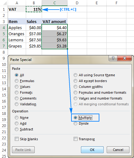
- Copy the numbers you want to multiply in the column where you want to output the results. In this example, we copy sales values (B4:B7) to the VAT column (C4:C7) because we don't want to override the original sales numbers.
- Input the constant number to multiply by in some empty cell, say B1. At this point, your data will look similar to this:

- Select the cell with the constant number (B1), and press Ctrl + C to copy it to the clipboard.
- Select the cells you want to multiply (C4:C7).
- Press Ctrl + Alt + V, then M, which is the shortcut for Paste Special > Multiply, and then press Enter.
Or, right-click the selection, choose Paste Special... in the context menu, select Multiply under Operations, and click OK.

Either way, Excel will multiply each number in the range C4:C7 by the value in B1 and return the results as values, not formulas:

Note. In some situations, you may need to reformat the Paste Special results. In the above example, we multiplied a column of numbers by percentage, and Excel formatted the results as percentages, while they should be numbers. To fix this, select the resulting cells and apply the desired Number Format to them, Currency in this case.
Multiply a column by a number with Ultimate Suite for Excel
Like Paste Special, this multiplication method returns values rather than formulas. Unlike Paste Special, Ultimate Suite for Excel is user-friendly and intuitive. Here's how you can multiply a column of numbers by another number in a couple of clicks:
- Select all cells that you want to multiply. If you'd like to keep the original values, copy them to another column where you want to get the results, and select those cells.
- On the Excel ribbon, go to the Ablebits Tools tab > Calculate group.
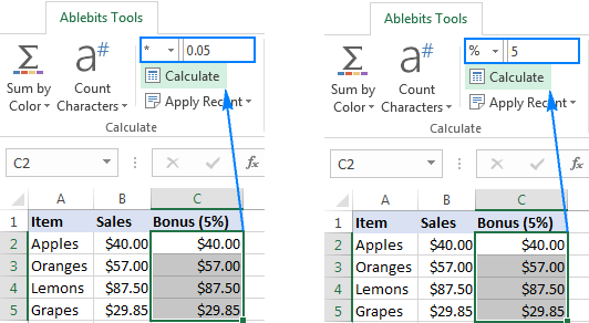
- Select the multiply sign (*) in the Operation box, type the number to multiply by in the Value box, and click the Calculate button.
As an example, let's calculate the 5% bonus on our sales. For this, we copy the sales values from column B to column C, and then either:
- Select the multiply sign (*) in the Operation box, and type 0.05 in the Value box (0.05 represents 5% because 5 percent is five parts of a hundred).
- Select the percent sign (%) in the Operation box, and type 5 in the Value box.

Both methods do multiplication right and produce identical results:

Unlike Excel's Paste Special feature, the Ultimate Suite retains the original Currency format, so no further adjustments to the results are required. If you are curious to try Ultimate Suite's calculation options in your worksheets, you are welcome to download an evaluation version by using the link below.
I thank you for reading and hope to see you on our blog next week!
Available downloads
Excel Multiply Columns - formula examples (.xlsx file)
Ultimate Suite - 14-day trial version (.exe file)
 by
by
30 comments
If you want to multiply by 2 the array A1:A10 (which holds the numbers 1,2,3,...10)
then there are at least 3 methods:
1) =A1:A10*2
2) =MMULT(A1:A10,2)
3) =BITLSHIFT(A1:A10,1)
Thank you so much I knew most of the keys I just forgot for a while lols
you do realize that none of this works?
okay me, i have number in AO I want Z to have this number but 10% added. How?
Hello Christoph,
To make sure all the formulas work as described, you can download our practice workbook and take a look at the examples.
As for your task, assuming your data begins in row 2, enter the below formula in Z2, and then drag it down through as many cells as needed:
=AO2+(AO2*0.1)
Hi!
Have you tried the ways described in this blog post? If they don’t work for you, then please describe your task in detail, I’ll try to suggest a solution.
All I have to say is huh?
Hi,
I just want to add column 1 and column 2 for a total in Colum 3. I am sure there is an easy calculation for this please help!
I would like to also find one to calculate ages. Column 1 date format and Column 2 the age. Please help!
thank you
Hello!
Please check out this article to learn how to calculate age in Excel.
I have 4 columns of 3 numbers each. I'd like to multiply each of the numbers in the first column by each of the numbers in the 2nd, 3rd, and 4th columns. To illustrate, I'd like to calculate A1*B1*C1*D1, and then calculate A1*B1*C1*D2, and then A1*B1*C1*D3 all the way to A3*B3*C3*D3. Any ideas?
can excel multiply between two number ranges? so if cell c4 "$360.00" is the bonus number and it is multiplied between 85%-100% but if the % is below 85% it needs to = 0 and if its above 100% it needs to = $360
Hello!
I’m sorry but your task is not entirely clear to me. Could you please describe it in more detail? What result do you want to get? Give an example of the source data and the expected result.
Totally appreciate your work, helped a lot ^_^ .
Suppose I have a data set in A and B. I want data from B to be multiplied by a multilplier depending on the value in column b. I have sorted the Column A by using Unique function. I am unable to do the rest.
Hello Shalini!
I think you need to use the IF function. Read more about this on our blog here. If you describe your problem in more detail, I will try to give you more detailed recommendations.
Thanks a ton
Hello,
I am trying to create a formula that will multiply certain numbers within a range (1-9) by specific numbers. For example if there is a 1 in a cell, I would like that to be multiplied by 24, if there is the number 2 in a cell I would like that to be multiplied by 13.5, if the number 3 is found in a cell I would like that to be multiplied by 10, the number 4 to be multiplied by 8.5, number 5 multiplied by 7.4, number 6 multiplied by 6.67, number 7 multiplied by 6.29, number 8 multiplied by 5.88, and number 9 multiplied by 5.56.
Essentially I am looking for this formula to convert numbers 1-9 to a scale of 50 and I am struggling with how to do that using conventional formulas found in excel or google sheets.
Anything you can do to help would be greatly appreciated. Thank you!
This is explanation is the best so far, the others were confusing. Thank you!
Thank you - that's the best explanation I have ever been given. Easy to follow and understand
Thank you
($L$2:$AH$2)*($L3:$AH3>0)
In the expression above, for each resulting cell, is a value only selected from array2 for each array2 / array3 combination where the array3 cell is greater than 0?
Thank you.
BEST EXPLANATION YET! THANKS!
I want to multiply column J2-J10 with K2-K10 and get a sum
then multiply J2-J10 with L2-L10 and get a sum
when I copy formula it does not keep j2-j10 consistent it shifts to the next column.
kindly help
is it possible to have result of multiplication in two cells
ie., C1*D1, result in E1 and F1 especially for splitting the currency. For Eg. 3.50*1, result to be appeared as 3 in E1 and 50 in F1
Sure! One way to do it is using this formula for E1 =TRUNC(C1*D1) and this other formula for F1 =ROUNDUP(((C1*D1)-E1)*100,0)
You may want to set column F to display no decimals.
Hi, I'm trying to calculate a formula which allow me to multiply one column by another column without the limit of ranges. For example, I would like to multiply each cell in column D by each corresponding cell in column E and have the product populated in column F. I have not found a useful formula for this as of yet. Please let me know if you have one.
Thank you.
Hello, did you ever receive an answer to your question? About not limiting the formula to a specific range of cells?
Thank you so much Svetkana, it is wery helpful thanks once again