In the recent couple of articles, we've looked at different ways to remove characters from strings in Excel. Today, we'll investigate one more use case - how to delete everything before or after a specific character.
Delete text before, after or between 2 characters with Find & Replace
For data manipulations in multiple cells, Find and Replace is the right tool. To remove part of a string preceding or following a specific character, these are the steps to perform:
- Select all the cells where you want to delete text.
- Press Ctrl + H to open the Find and Replace dialog.
- In the Find what box, enter one of the following combinations:
- To eliminate text before a given character, type the character preceded by an asterisk (*char).
- To remove text after a certain character, type the character followed by an asterisk (char*).
- To delete a substring between two characters, type an asterisk surrounded by 2 characters (char*char).
- Leave the Replace with box empty.
- Click Replace all.
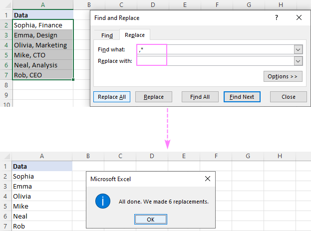
For example, to remove everything after a comma including the comma itself, put a comma and an asterisk sign (,*) in the Find what box, and you'll get the following result:

To delete a substring before a comma, type an asterisk, a comma, and a space (*, ) in the Find what box.
Please notice that we are replacing not just a comma but a comma and a space to prevent leading spaces in the results. If your data is separated by commas without spaces, then use an asterisk followed by a comma (*,).

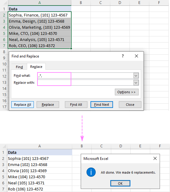
To delete text between two commas, use an asterisk surrounded by commas (,*,).

Tip. If you'd rather have the names and phone numbers separated by a comma, then type a comma (,) in the Replace with field.
Remove part of text using Flash Fill
In modern versions of Excel (2013 and later), there is one more easy way to eradicate text that precedes or follows a specific character - the Flash Fill feature. Here's how it works:
- In a cell next to the first cell with your data, type the expected result and press Enter.
- Start typing an appropriate value in the next cell. Once Excel feels the pattern in the values you are entering, it will display a preview for the remaining cells following the same pattern.
- Hit the Enter key to accept the suggestion.
Done!

Remove text using formulas
In Microsoft Excel, many data manipulations performed by using inbuilt features can also be accomplished with a formula. Unlike the previous methods, formulas do not make any changes to the original data and give you more control over the results.
How to remove everything after a specific character
To delete text after a particular character, the generic formula is:
Here, we use the SEARCH function to get the position of the character and pass it to the LEFT function, so it extracts the corresponding number of characters from the start of the string. One character is subtracted from the number returned by SEARCH to exclude the delimiter from the results.
For example, to remove part of a string after a comma, you enter the below formula in B2 and drag it down through B7:
=LEFT(A2, SEARCH(",", A2) -1)

How to remove everything before a specific character
To delete part of a text string before a certain character, the generic formula is:
Here, we again calculate the position of the target character with the help of SEARCH, subtract it from the total string length returned by LEN, and pass the difference to the RIGHT function, so it pulls that many characters from the end of the string.
For example, to remove text before a comma, the formula is:
=RIGHT(A2, LEN(A2) - SEARCH(",", A2))
In our case, the comma is followed by a space character. To avoid leading spaces in the results, we wrap the core formula in the TRIM function:
=TRIM(RIGHT(A2, LEN(A2) - SEARCH(",", A2)))

Notes:
- Both of the above examples assume that there is only one instance of the delimiter in the original string. If there are multiple occurrences, text will be removed before/after the first instance.
- The SEARCH function is not case-sensitive, meaning it makes no difference between lowercase and uppercase characters. If your specific character is a letter and you want to distinguish the letter case, then use the case-sensitive FIND function instead of SEARCH.
How to delete text after Nth occurrence of a character
In situation when a source string contains multiple instances of the delimiter, you may have a need to remove text after a specific instance. For this, use the following formula:
Where n is the character's occurrence after which to remove text.
The internal logic of this formula requires using some character that is not present anywhere in the source data, a hash symbol (#) in our case. If this character occurs in your data set, then use something else instead of "#".
For example, to remove everything after the 2nd comma in A2 (and the comma itself), the formula is:
=LEFT(A2, FIND("#", SUBSTITUTE(A2, ",", "#", 2)) -1)

How this formula works:
The key part of the formula is the FIND function that calculates the position of the nth delimiter (comma in our case). Here's how:
We replace the 2nd comma in A2 with a hash symbol (or any other character that does not exist in your data) with the help of SUBSTITUTE:
SUBSTITUTE(A2, ",", "#", 2)
The resulting string goes to the 2nd argument of FIND, so it finds the position of "#" in that string:
FIND("#", "Emma, Design# (102) 123-4568")
FIND tells us that "#" is the 13th character in the string. To know the number of characters preceding it, just subtract 1, and you'll get 12 as the result:
FIND("#", SUBSTITUTE(A2, ",", "#", 2)) - 1
This number goes directly to the num_chars argument of LEFT asking it to pull the first 12 characters from A2:
=LEFT(A2, 12)
That's it!
How to delete text before Nth occurrence of a character
The generic formula to remove a substring before a certain character is:
For example, to strip off text before the 2nd comma in A2, the formula is:
=RIGHT(SUBSTITUTE(A2, ",", "#", 2), LEN(A2) - FIND("#", SUBSTITUTE(A2, ",", "#", 2)) -1)
To eliminate a leading space, we again use the TRIM function as a wrapper:
=TRIM(RIGHT(SUBSTITUTE(A2, ",", "#", 2), LEN(A2) - FIND("#", SUBSTITUTE(A2, ",", "#", 2))))

How this formula works:
In summary, we find out how many characters are after the nth delimiter and extract a substring of the corresponding length from right. Below is the formula break down:
First, we replace the 2nd comma in A2 with a hash symbol:
SUBSTITUTE(A2, ",", "#", 2)
The resulting string goes to the text argument of RIGHT:
RIGHT("Emma, Design# (102) 123-4568", …
Next, we need to define how many characters to extract from the end of the string. For this, we find the position of the hash symbol in the above string (which is 13):
FIND("#", SUBSTITUTE(A2, ",", "#", 2))
And subtract it from the total string length (which equals to 28):
LEN(A2) - FIND("#", SUBSTITUTE(A2, ",", "#", 2))
The difference (15) goes to the second argument of RIGHT instructing it to pull the last 15 characters from the string in the first argument:
RIGHT("Emma, Design# (102) 123-4568", 15)
The output is a substring " (102) 123-4568", which is very close to the desired outcome, except a leading space. So, we use the TRIM function to get rid of it.
How to remove text after the last occurrence of a character
In case your values are separated with a variable number of delimiters, you may want to remove everything after the last instance of that delimiter. This can be done with the following formula:
Suppose column A contains various information about employees, but the value after the last comma is always a telephone number. Your goal is to remove phone numbers and keep all other details.
To achieve the goal, you can remove text after the last comma in A2 with this formula:
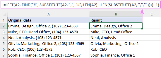
=LEFT(A2, FIND("#", SUBSTITUTE(A2, ",", "#", LEN(A2) - LEN(SUBSTITUTE(A2, ",","")))) -1)
Copy the formula down the column, and you'll get this result:

How this formula works:
The gist of the formula is that we determine the position of the last delimiter (comma) in the string and pull a substring from left up to the delimiter. Getting the delimiter's position is the trickiest part, and here's how we handle it:
First, we find out how many commas there are in the original string. For this, we replace each comma with nothing ("") and serve the resulting string to the LEN function:
LEN(SUBSTITUTE(A2, ",",""))
For A2, the result is 35, which is the number of characters in A2 without commas.
Subtract the above number from the total string length (38 characters):
LEN(A2) - LEN(SUBSTITUTE(A2, ",",""))
… and you will get 3, which is the total number of commas in A2 (and also the ordinal number of the last comma).
Next, you use the already familiar combination of the FIND and SUBSTITUTE functions to get the position of the last comma in the string. The instance number (3rd comma in our case) is supplied by the above-mentioned LEN SUBSTITUTE formula:
FIND("#", SUBSTITUTE(A2, ",", "#", 3))
It appears that the 3rd comma is the 23rd character in A2, meaning we need to extract 22 characters preceding it. So, we put the above formula minus 1 in the num_chars argument of LEFT:
LEFT(A2, 23-1)
How to remove text before the last occurrence of a character
To delete everything before the last instance of a specific character, the generic formula is:
In our sample table, to eradicate text before the last comma, the formula takes this form:
=RIGHT(A2, LEN(A2) - FIND("#", SUBSTITUTE(A2, ",", "#", LEN(A2) - LEN(SUBSTITUTE(A2, ",","")))))
As a finishing touch, we nest it into the TRIM function to eliminate leading spaces:
=TRIM(RIGHT(A2, LEN(A2) - FIND("#", SUBSTITUTE(A2, ",", "#", LEN(A2) - LEN(SUBSTITUTE(A2, ",",""))))))

How this formula works:
In summary, we get the position of the last comma as explained in the previous example and subtract it from the total length of the string:
LEN(A2) - FIND("#", SUBSTITUTE(A2, ",", "#", LEN(A2) - LEN(SUBSTITUTE(A2, ",",""))))
As the result, we get the number of characters after the last comma and pass it to the RIGHT function, so it brings that many characters from the end of the string.
Custom function to remove text on either side of a character
As you have seen in the above examples, you can resolve almost any use case by using Excel's native functions in different combinations. The problem is that you need to remember of handful of tricky formulas. Hmm, what if we write our own function to cover all the scenarios? Sounds like a good idea. So, add the following VBA code to your workbook (the detailed steps to insert VBA in Excel are here):
Our function is named RemoveText and it has the following syntax:
Where:
String - is the original text string. Can be represented by a cell reference.
Delimiter - the character before/after which to remove text.
Occurrence - the instance of the delimiter.
Is_after - a Boolean value that indicates on which side of the delimiter to remove text. Can be a single character or a sequence of characters.
- TRUE - delete everything after the delimiter (including the delimiter itself).
- FALSE - delete everything before the delimiter (including the delimiter itself).
Once the function's code is inserted in your workbook, you can remove substrings from cells using compact and elegant formulas.
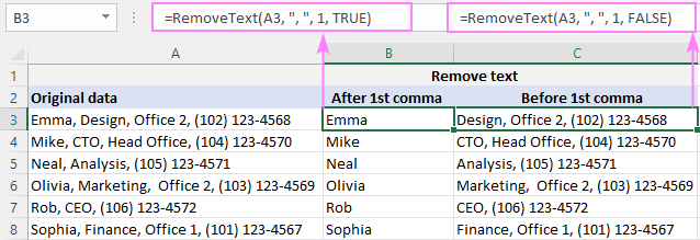
For example, to erase everything after the 1st comma in A2, the formula in B2 is:
=RemoveText(A3, ", ", 1, TRUE)
To delete everything before the 1st comma in A2, the formula in C2 is:
=RemoveText(A3, ", ", 1, FALSE)
Since our custom function accepts a string for the delimiter, we put a comma and a space (", ") in the 2nd argument to spare the trouble of trimming leading spaces afterwards.

Our custom function works beautifully, doesn't it? But if you think it's the comprehensive solution, you haven't seen the next example yet :)
Delete everything before, after or between characters
To get even more options for removing individual characters or text from multiple cells, by match or position, add our Ultimate Suite to your Excel toolbox.
Here, we'll take a closer look at the Remove by Position feature located on the Ablebits Data tab > Text group > Remove.

Below, we will cover the two most common scenarios.
Remove everything before or after certain text
Suppose all your source strings contain some common word or text and you wish to delete everything before or after that text. To have it done, select your source data, run the Remove by Position tool, and configure it like shown below:
- Select the All characters before text or All characters after text option and type the key text (or character) in the box next to it.
- Depending on whether uppercase and lowercase letters should be treated as different or the same characters, check or uncheck the Case-sensitive box.
- Hit Remove.
In this example, we are removing all characters preceding the word "error" in cells A2:A8:

And get exactly the result we are looking for:

Remove text between two characters
In situation when irrelevant information is between 2 specific characters, here's how you can quickly delete it:
- Choose Remove all substrings and type two characters in the below boxes.
- If the "between" characters should be removed too, check the Including delimiters box.
- Click Remove.

As an example, we delete everything between two tilde characters (~), and get the perfectly cleaned strings as the result:

To try other useful features included with this multi-functional tool, I encourage you to download an evaluation version at the end of this post. Thank you for reading and hope to see you on our blog next week!
Available downloads
Remove first or last characters - examples (.xlsm file)
Ultimate Suite - trial version (.exe file)
 by
by
22 comments
Thank you so much, that helped tremendously.
This is what my string looks like ", South Korea". How do I clean this without it affecting other cells? For it to be "South Korea". There are plenty of them like this. Have it in mind that 2 or more countries can be in one cell separated by a comma and space.
Hi! If I understand your task correctly, this article may be helpful: How to remove special (unwanted) characters from string in Excel
I have situation like this, in a column number and text are combine and multiply by the price but it is error when i do.
can you remove the text
25 pcs x 30.00 = 750.00
10 bxs x 100.00 = 1000.00
Hi! You can convert text to a formula only using a VBA macro. However, if you are using data from multiple cells, you can first extract all numbers from text “25 pcs” and then multiply them by value in another cell, for example, 30. For example:
=LEFT(A2, MATCH(FALSE, ISNUMBER(MID(A2, ROW(INDIRECT("1:"&LEN(A2)+1)), 1) *1), 0) -1) * B2
For the detailed instructions, please see: Extract number from text string.
For your data, you can extract all the digits before the first space and then multiply by the number.
=LEFT(A2, SEARCH(" ",A2)-1) * B2
Read more: Get text before a specific character
Hi, I'm looking to extract all text between French brackets "{" and "}" within a string... including the brackets themselves, and the extra space.
Example
Outside {corner property} 600 Anywhere Ave, Nowhere... becomes Outside 600 Anywhere Ave, Nowhere
Thanks in advance for any help you can offer.
Hi! To remove some of the text between delimiters from a text string, use the TEXTBEFORE and TEXTAFTER functions.
=TEXTBEFORE(A1,"{")&TEXTAFTER(A1,"}")
If these functions are not available to you, use this guide: Excel substring: how to extract text from cell.
=LEFT(A1, SEARCH("{",A1)-1)&RIGHT(A1,LEN(A1)-SEARCH("}",A1))
Sorted. Sorry I should have read more fully previous explanations!
=TEXTBEFORE(A1,"{")&TEXTAFTER(A1,"} ")
Thanks for sharing your knowledge, I wasn't even aware of the TEXTBEFORE/AFTER functions.
Hi
I need to extract text only from cells (remove numbers or others in cells)
192938-GDASa
I need 192938 only
Hi! We have a special tutorial on this. Please see: Extract number from text string.
For example:
=LEFT(A1, MATCH(FALSE, ISNUMBER(MID(A1, ROW(INDIRECT("1:"&LEN(A1)+1)), 1) *1), 0) -1)
KF68SDX - how to split text and numbers
Hi! You can extract numbers from text in a cell using any of methods described in this article: How to extract number from string in Excel.
To extract all characters from the text, you can replace numbers with blanks using the SUBSTITUTE function:
=SUBSTITUTE((CONCAT(IF(NOT(ISNUMBER(--MID(A1,ROW($1:$50),1))),MID(A1,ROW($1:$50),1),"")))," "," ")
INV9999999 / 123456 This is cell. I need to get the invoice # in one cell and the 123456 in another cell. Can you help me?
Hi! You can find the examples and detailed instructions here: How to split text string in Excel by comma, space, character or mask. Try the following formulas:
=LEFT(A2, SEARCH("/",A2,1)-1)
=MID(A2, SEARCH("/",A2,1)+1,50)
You can also use the new TEXTSPLIT function to split the text by cells:
=TEXTSPLIT(A2,"/")
Hello! I am trying to remove text before a character, but the data has multiple characters.
Ex: My data looks like
123A
123B
123C
I would like to remove the text before A, B, C.
I am currently using:
=LEFT(cell, SEARCH("A", cell) -1)
but this only works for one character at a time.
Hi! Your formula does not remove the text before the character, it extracts it. To extract the text before three different characters, you can combine 3 formulas using the IFERROR function.
=IFERROR(LEFT(A1,SEARCH("A",A1)-1), IFERROR(LEFT(A1,SEARCH("B",A1)-1), LEFT(A1,SEARCH("C",A1)-1)))
I recommend reading this guide: Excel IFERROR function with formula examples.
I hope it’ll be helpful. If this is not what you wanted, please describe the problem in more detail.
Hi, I need your help! I need to remove part of the text in multiple cells in excel/google sheet.
Exp: Employee: Jose Pinesa. I need to romove Employee:
How can I do that to save me time?
Thank you
Hi! You can delete part of the text using the SUBSTITUTE function:
=SUBSTITUTE(A1,"Employee:","")
"WORK COMPLETEDÂ
Â
BLADDER REPAIREDÂ Â "
how do i make above characters need to be like " WORK COMPLETED BLADDER REPAIRED"
please assist me
Hi! If these values are written in different cells, to merge the text, use this guide: Excel CONCATENATE function to combine strings, cells, columns.
If text is written in multiple rows of the same cell, use these instructions: How to remove carriage returns (line breaks) from cells in Excel.
How may I eliminate or removed the text from the time? Example: 8:30 am Work from Home...
Thank you.
Hi! Find the first space with the SEARCH function and extract the time with the LEFT function. The TIMEVALUE function will help you convert text to time.
=TIMEVALUE(LEFT(A1,SEARCH(" ",A1)))