From this short tip you will learn how to quickly sort cells by background and font color in Excel 365 - Excel 2010 worksheets.
Last week we explored different ways to count and sum cells by color in Excel. If you've had a chance to read that article, you may wonder why we neglected to show how to filter and sort cells by color. The reason is that sorting by color in Excel requires a bit different technique, and this is exactly what we are doing to do right now.
Sort by cell color in Excel
Sorting Excel cells by colour is the easiest task compared to counting, summing and even filtering. Neither VBA code nor formulas are needed. We are simply going to use the Custom Sort feature available in all versions of Excel 365 through Excel 2007.
- Select your table or a range of cells.
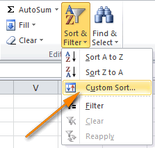
- On the Home tab > Editing group, click the Sort & Filter button and select Custom Sort…
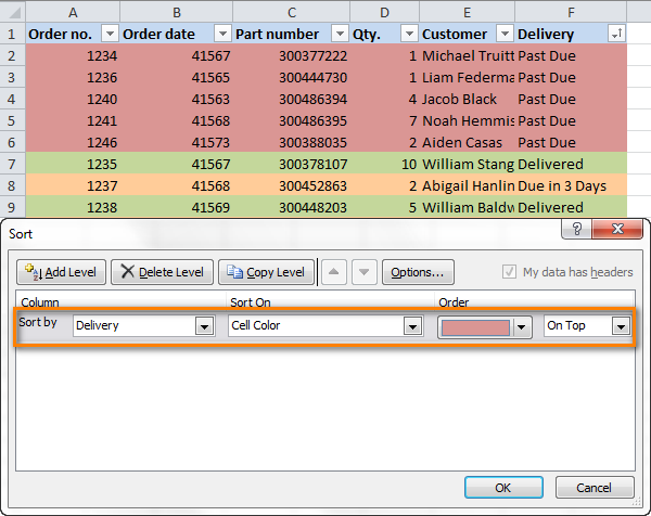
- In the Sort dialog window, specify the following settings from left to right.
- The column that you want to sort by (the Delivery column in our example)
- To sort by Cell Color
- Choose the color of cells that you want to be on top
- Choose On Top position
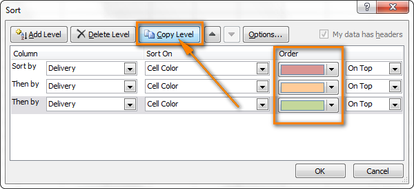
- Click the Copy Level button to add one more level with the same settings as the first one. Then, under Order, select the color second in priority. In the same way add as many levels as many different colors are in your table.
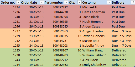
- Click OK and verify if your rows have got sorted by color correctly.
In our table, the "Past Due" orders are on top, then come "Due in" rows, and finally the "Delivered" orders, exactly as we wanted them.
Tip: If your cells are colored with many different colors, it is not necessary to create a formatting rule for each and every one of them. You can create rules only for those colors that really matter for you, e.g. "Past due" items in our example and leave all other rows in the current order.

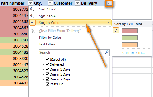
If sorting cells by only one color is what you are looking for, then there's even a quicker way. Simply click on the AutoFilter arrow next to the column heading you want to sort by, choose Sort by color from the drop down menu, and then select the color of cells that you want to be on top or at the bottom. BTW, you can also access the "Custom Sort" dialog from here, as you can see in the right hand part of the screenshot below.
Sort cells by font color in Excel
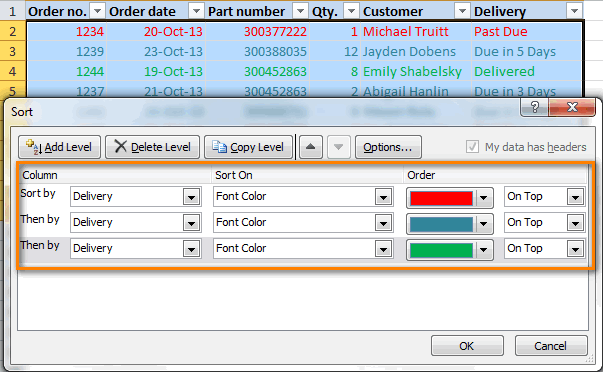
In fact, sorting by font colour in Excel is absolutely the same as sorting by background color. You use the Custom Sort feature again (Home > Sort & Filter > Custom Sort…), but this time choose Font Color under "Sort on", as shown in the screenshot below.
If you want to sort by just one font color, then Excel's AutoFilter option will work for you too:

Apart from arranging your cells by background colour and font color, there may a few more scenarios when sorting by color comes in very handy.
Sort by cell icons
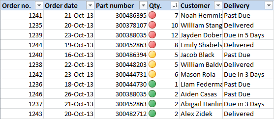
For example, we can apply conditional formatting icons based on the number in the Qty. column, as shown in the screenshot below.
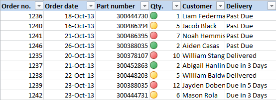
As you see, big orders with quantity more than 6 are labeled with red icons, medium size orders have yellow icons and small orders have green icons. If you want the most important orders to be on top of the list, use the Custom Sort feature in the same way as described earlier and choose to sort by Cell Icon.
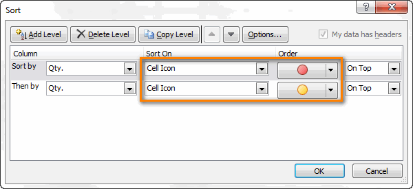
It is enough to specify the order of two icons out of 3, and all the rows with green icons will get moved to the bottom of the table anyway.
How to filter cells by color in Excel
If you want to filter the rows in your worksheet by colors in a particular column, you can use the Filter by Color option available in Excel 365 - Excel 2016.
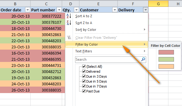
The limitation of this feature is that it allows filtering by one color at a time. If you want to filter your data by two or more colours, perform the following steps:
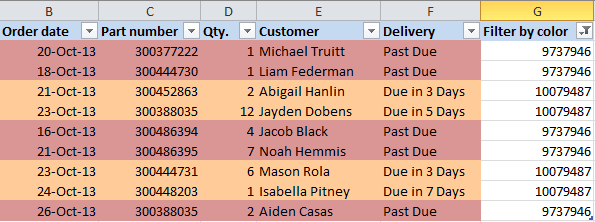
- Create an additional column at the end of the table or next to the column that you want to filter by, let's name it "Filter by color".
- Enter the formula
=GetCellColor(F2)in cell 2 of the newly added "Filter by color" column, where F is the column congaing your colored cells that you want to filter by. - Copy the formula across the entire "Filter by color" column.
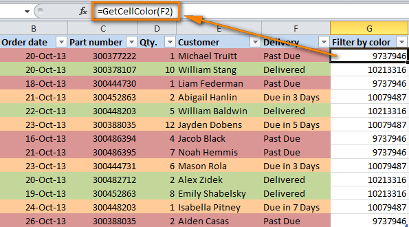
- Apply Excel's AutoFilter in the usual way and then select the needed colors in the drop-down list.
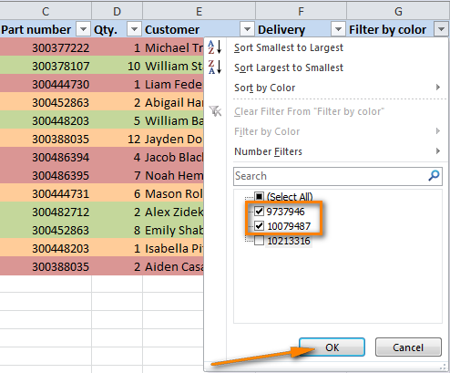
As a result, you will get the following table that displays only the rows with the two colors that you selected in the "Filter by color" column.
And this seems to be all for today, thank you for reading!
 by
by
46 comments
Hi, I was curious as I didn't see this and can't figure it out yet. Can you sort 8 columns for color at one time? Or only one at at time? This is what I would really love to be able to do.
Thank you.
Anne
Respected svetlana i want to share and ask solution of of one excel formula issue is that... if there are multiple column in an exam formula and i want the column where the word PASS is written then how to get data of these relevent coulmns
Hello!
Your question is not very clear, but maybe this article will be helpful: Excel INDEX MATCH MATCH and other formulas for two-way lookup. If this does not help, explain the problem in detail.
Hi Everyone,
I have a problem, i have 10 columns data and i have sorted this data using one column. But Now i want to revert to original positions of each value. Please tell. It's very very important. I have tried "Ctrl+Z" command, but because i have closed and opened excel files many time, it is now useless. I have also tried Clearing filter option, but nothing happens, it just disappears arrow on drop down of filter and does not revert my values to original state. Please guide how to get rid of this problem.
I have two columns with about six colors of cells (corresponding rows of cells for each column are the same color) but when I try to custom sort by color, the only color option I have is "no color". No other color shows up in the drop down. I filled the cells using the fill bucket. Do you have any idea why the colors of the cells aren't recognized? I highlighted one column, both columns etc. I can sort these same columns other ways but not by color... THANKS! Frustrated!
Thank you very much for a clearly stated tutorial! Just what I needed!
Not getting option sort by colour on Microsoft Excel mobile app.....Pls.help..
Hello, can I filter the whole sheet by color? I have an spread sheet with a lot of data, but when i completed my items, I just want to see just what I mark on color.
thank you in advance
to do this all the merged cells must be same size,
please advise
Hello,
How To Extract cell values based On cell Color for example in a 3×3 matrix(1st coloumn 1st cell and 3rd coloumn 2nd cell are filled with blue and the rest is filled with yellow), in this case lusting only the cell values filled with blue colour and listing this separately in the same excel?
Is there any way to save my 5 level color sort so that I can use this on a number of worksheets in the same workbook? It appears you can't a color sort in a custom list
Hello, I am wanting to pull data by color. For example, if column A is made up of blank cells that are green, but when a date is added to the cell we turn it orange until the item is returned then the date is turned green again. Can you get it to pull the number of orange cells in Column A?
Secondly, can you get it to pull the number of green cells with data entered?
Hi,
is it possible in excel automatically ignore that the cell colored for pivot table,
for ex: if I entered 12,13,14 number in column B and in the C column I entered 12, and 13 only then I will coloring the cell using conditional format (Duplicate value) then the remain is 14 that 14 only should come to the Pivot table??
Thanks And Best Regards
Ali
Wow thank you for this. I have multiple cell colors and you just made my life so much easier.
After I select "font color" under the "Sort On" column I attempt to select a color under "Order" but the only option available to select is "Automatic". Any idea what I am doing incorrectly?
Hello,
Perhaps, there are no cells with another font color except Automatic in the column you select for sorting.
Hi
On the drop down menu at the top of the column the "sort by..." feature does not come up, just "custom sort". How do I get color sort back?
Thanks
Hi Kevin,
Please check that there are cells with more than one font or fill color in the selected column.
I appreciate the effort put into explaining the features present in Excel.
Thanks.
We have data in a spreadsheet that has been subtotaled. There are certain lines that we want to look at and have changed the cell color for that data. But now we can't seem to sort by the cell color. Is that because the data is already subtotaled?
please tell me how to exit from this function
Gud work
my excel worksheet cell have colors in it, not in all. But the problem is i cannot see the cell color when try to sort by color. Why?