What does #SPILL mean in Excel? It's an error that occurs when a formula is unable to populate multiple cells with the calculated results. To learn what can trigger this error and how you can resolve it, please keep reading.
Just imagine this: you upgraded to Microsoft Office 365 with the latest Excel updates and for some reason the tried and tested formulas you've been using for years have suddenly stopped working. Whatever you do, you are now getting a #SPILL error. Does anyone know what it means? Of course, we do, and you'll get your solution in a moment :)
What does #SPILL mean in Excel?
Generally, a #SPILL! error occurs when a formula produces multiple results but cannot output them all on the sheet.
Before we dive into specific use cases, let's get a general understanding of spilling in Excel.
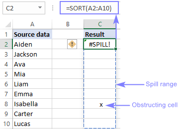
With the launch of dynamic arrays in Excel 365, any formula that produces multiple calculation results automatically "spills" those results into neighboring cells. Please notice, any formula, even the ones that were not initially designed to handle arrays. A range of cells containing the results is called a spill range. And if something on the sheet prevents filling that range, a #SPILL! error occurs.
For the most part, this behavior is understandable and predictable. For instance, if your formula is expected to return more than one value, but the nearby cells are filled with some other data, simply delete that data, and an error will be gone.
But sometimes the reasons are not so obvious and therefore confusing. Perhaps, one or more cells in the spilled area contain a space or a non-printing character invisible to a human eye. Or the same formula copied across the entire column blocks a spill range. Or, you might have run into one of the very few features that do not support dynamic arrays. To fix an error, you'll have to investigate each case individually and determine the root of the problem.
How to fix #SPILL! error in Excel
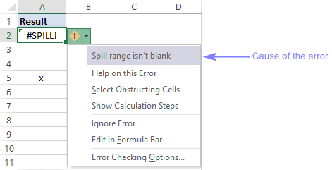
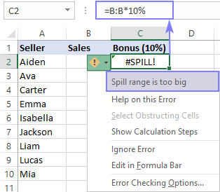
As mentioned above, a #SPILL! error might be caused by various reasons. To know the exact root of the problem, click the warning icon (a yellow diamond with an exclamation point), and read the message in the first line highlighted in grey:
Once you determined the cause, please find the corresponding example below with the detailed instructions on how to resolve that particular case.
Spill range isn't blank
Reason: The area to be populated with the formula results contains non-empty cells.
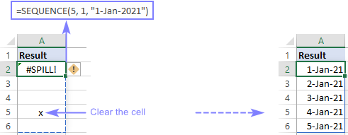
Solution: Clear the expected spill range.
In a simplest scenario, just click the formula cell and you will see a dashed border indicating the spill range boundaries - any data inside it is an obstacle. So, either remove the existing data from the spill area or move the formula to another location where there is no blockage.
In some situations, however, a spill range may look blank, but in fact it is not. The problem may be in invisible characters such as a space lurking in some cells, or formulas returning an empty string.
To detect such cells, click a warning sign, and you will see this explanation - Spill range isn't blank. Underneath it, there are a number of options. Click Select Obstructing Cells, and Excel will show you which cells prevent the formula from spilling.
In the screenshot below, the obstructing cell is A6, which contains an empty string ("") returned by the formula.
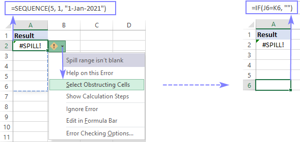
To clear blocking cells, go to the Home tab > Editing group, and click Clear > Clear All.
Spill range contains merged cells
Reason: Spilling does not work with merged cells.
Solution: Unmerge cells in the spilled area or move the formula to another location that has no merged cells.
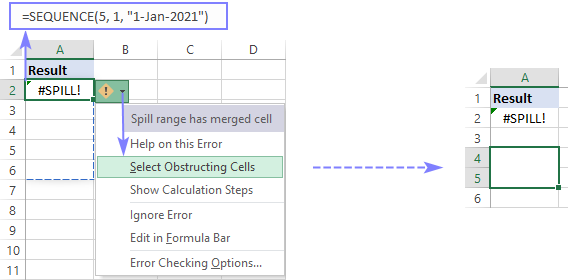
In case there are one or more merged cells in a projected spilled array, the following error message is displayed - Spill range has merged cell.
If you have difficulties detecting the merged cells visually, make use of Select Obstructing Cells option to jump to the problematic cells:
Spill range in table
Reason: Dynamic arrays are not supported in Excel tables.
Solution: Convert the table to a normal range or place the formula outside the table to allow it to spill. It's not quite clear why dynamic array formulas do not work from within Excel tables (maybe because of the specific syntax of structured references), but anyway these two very useful things do not get along :(
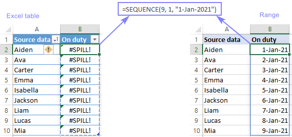
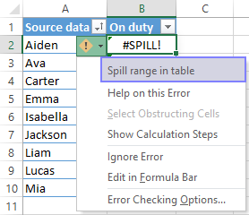
To confirm the root cause of the problem, click an icon with an exclamation mark, and you will see this text in the first line - Spill range in table.
In this case, the best thing you could do is to convert table to range. For this, right-click anywhere within the table, and then click Table > Convert to Range. Alternatively, you can move your formula beyond the table boundaries.
Spill range is unknown
Reason: Excel is unable to establish the size of the spilt array.
Solution: Try to work out a different formula for your task.
When using volatile functions such as RANDARRAY, RAND or RANDBETWEEN in combination with dynamic array functions, a #SPILL error may occur because the array returned by a volatile function changes between the spreadsheet's calculations and the "wrapper" function cannot determine its size.
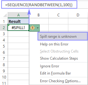
In such situation, an error message says - Spill range is unknown.
For example, the following formula throws a #SPILL! error because the RANDBETWEEN output continuously changes and SEQUENCE does not know how many values to generate:
=SEQUENCE(RANDBETWEEN(1,100))
Spill range is too big
Reason: Excel is unable to output a spilt array as it extends beyond the spreadsheet edges.
Solution: Instead of calculating entire columns, reference a used range, a single cell, or add the @ operator to perform implicit intersection.
It is the most complex case and depending on your goal and the worksheet's structure you may need to adjust your formulas differently. Here, we are going to demonstrate a general approach on a very simple example.
Supposing you have a list of numbers in column B, and in column C you wish to return 10% of those numbers.
In traditional Excel 2019 and earlier, the following formula worked without a hitch (in the left part of the image below, it's in cells C2 through C7):
=B:B*10%
In dynamic Excel 365, the same formula triggers a #SPILL error.
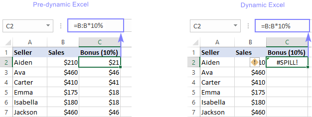
The cause of the error is Spill range is too big.
Why is the formula broken in new Excel? Because implicit intersection is no longer silently performed in the background. The term sounds mysterious, but the logic behind it is quite simple - reduce multiple values to a single value.
In pre-365 versions, that was the default behavior of Excel - since a cell could only contain one value, a formula was forced to return a single result. In our example, even though we supply a whole column (B:B), Excel processes just one value on the same row as the formula. So, the formula in C2 calculates 10% of the value in B2, the formula in C3 calculates 10% of the value in B3, and so on.
In dynamic array Excel, the default behavior is different - any formula that can potentially return multiple results automatically spills them onto to the worksheet. In our case, Excel multiplies each cell in column B by 10%, gets over a million results (more precisely 1,048,576), tries to output all of them in column C beginning in C2, but reaches the end of the worksheet grid - hence a #SPILL error. Guess what happens if we put the formula in C1? Yep, it will work because this time there are enough cells to fill - the spill range will occupy exactly 1,048,576 cells!
Solution 1. Refer to ranges rather than columns
This is a very reasonable approach - instead of referencing entire columns, reference only the relevant data. Apart from fixing a #SPILL error, it also helps to save Excel resources and improve performance.
For our sample dataset, the formula is:
=B2:B10*10%
The formula is entered just in one cell (C2). The result is a dynamic array that spills into multiple cells automatically:

Note. Because dynamic arrays are not supported in Excel tables, this solution only works within a normal range.
Solution 2. Calculate a single cell and copy the formula down
It is the traditional approach - reference one cell on the same row and copy the formula down.
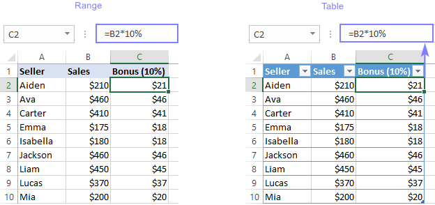
In our case, the below formula goes to C2, and then you drag it down through C10:
=B2*10%
Unlike dynamic array formulas, this conventional formula style works in ranges and tables equally well:
Solution 3. Apply implicit intersection
This approach is a bit more complicated - use the implicit intersection operator (@ symbol) which was introduced in Excel 365 as part of the dynamic arrays update.
In your formula, insert the @ character where you want to reduce an array or a range to a single value, e.g. before a range/column/row reference, function or expression. Enter the formula in the topmost cell, and then drag it down across as many rows as needed.
For our sample dataset, the formula takes this shape:
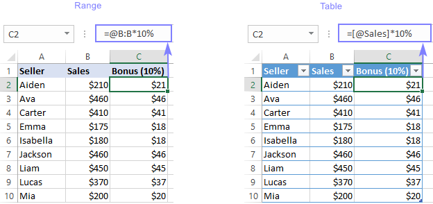
=@B:B*10%
Since the result is a single value, not a dynamic array, this formula can be used both in ranges and tables. In the latter case, however, a structured reference would be a more elegant and effective solution:
=[@Sales]*10%
To some extent, this explains why the "@" character occasionally appears in formulas created in older versions - to retain compatibility. Because in pre-dynamic Excel, formulas cannot spill into multiple cells, the implicit intersection operator secures the same behavior when the formula is imported in dynamic array Excel.
My personal advice is to use this approach with care because it disables a great new feature of Excel that is very efficient and helpful in many scenarios.
That's how to troubleshoot and fix a #SPILL error in Excel. In the incoming article, we are going to investigate and resolve this error in a few popular formulas such as VLOOKUP, INDEX MATCH, SUMIF, etc. Thank you for reading and please stay tuned!
 by
by
26 comments
i have spill on vlookup(=VLOOKUP(A2:A67;'PIVOT LEASE'!A5:B64;2;FALSE))
Hi! The vlookup_value argument in your VLOOKUP formula contains 65 values. Therefore, the formula returns 65 results.
In the column below the formula, there should be 64 empty cells.
If not, you will get an error.
I recommend reading this guide: Excel VLOOKUP function tutorial with formula examples.
Hello All,
I am working on a report in which I have to bring combined financial value from sheet1 to sheet2. I have unique IDs on sheet2, which have multiple row entries on sheet1. Currently, I have used sumproduct(filter()) to get the desired result but since filter() is a dynamic function, it slows me down.
Is there any alternate to this? I would be happy to share this sheet for better understanding and help.
Regards
Ahmad Rana
Hi! You can find the sum by condition without using the FILTER function. You can use these conditions directly in the SUMPRODUCT function as described in this manual: Excel SUMPRODUCT function with formula examples.
I hope it’ll be helpful. If something is still unclear, please feel free to ask.
Hello!
Thank you for this information, it's very insightful. Although, it doesn't necessarily help with my situation, and i want to see if someone could help me!
Say i have column A rows 1-10 Numbered sequentially 1,2,3,4.... and column B rows 1-10 corresponding with Column A. Then I have Column C rows 1-10 having the same id/numbers as column A, but they're not sequential eg: 2,6,4,8,1... and i have Column D corresponding to Column C. I want to the data in column A and column C to match, then grab the data from Column B and put it into Column E rows 1-10. I've done the formula "=IF(A1=C1:C10, B1, "")"
but if i try to do the same with "=IF(A2=C1:C10, B2, "")" it will give me a #SPILL because it's giving me all the rows. I've tried to do =INDEX but it gives me #REF. I'm struggling to find the correct solution, if you could please help me.
Since column B corresponds to A and A corresponds to C, column E will simply contain the values from column C.
Hello,
I am trying to take the value from one larger merged cell, and have it automatically fill into another NOT merged cell. This results in the spill error. How do i fix this without unmerging the cells in question (This is a format thing that can't be changed)
Hi!
Perhaps there is an array of values in the merged cell. Then it may cause an error.
Thank you so much for this article Svetlana. Saved my life this morning after we had to convert to dynamic Excel and none of my automated reports worked. What a pain but now resolved thanks to you and this @.
I know that my large excel file with 150 tabs has a #spill! error in it because I can see the opening message that spill resizing is occurring but I cannot locate the #spill! value or the cell causing the #spill!. Any suggestions? Thank you!
My formula is =TRIM(b2)&" "&TRIM(c2)&" "&d2 but when I enter it puts #SPILL (spill range is too big), how do I deal with this? Thank you!
Hello!
I can't reproduce your problem as I don't know what data is written in those cells. Please read the above article carefully. If this is not enough, describe the problem in more detail.
This feedback did me no good...I don't want excel to do anything at all...I just want to have a cell that I can place a value in from another tab and that's it...no cascading anything afterward...what a POS error
I'm using the formula =if(T20:T230=" ";" ";countif($U19$:U19;">0")+1) without any problem for quite a long period. However, with 365 it gives a #SPILL error.
Hello!
The expression T20:T230=” “ returns an array of 210 values. If there are data cells in the column below the formula, a #SPILL! error is returned.
$U19$:U19 - incorrect.
I’ll try to guess and offer you the following formula:
=IF(SUM(--(T20:T230=" "))=0," ",COUNTIF($U$19:U19,">0"))
I have solved the problem by adding @ in front of U20:U230
=if(@T20:T230=" ";" ";countif($U19$:U19;">0")+1)
This "function" is an absolute disaster!
I cannot understand how you cannot turn it off when the potential for errors is so large for something like this.
Bizzare! Suddenly this appears in an Excel 10 created workbook, used for years, and the sell is a simple "+" addition of a range name + the Sum() of a group of sequential cells in one column on another tab.
Some serious cursing (for me) was thrown at Msoft software engineers this morning.
The solution? Remove the "+_" symbol, and the added "@" and encase the range name and reference to cells on the other tab in a SUM() formula.
I HATE this Office 365. It is a MESS.
Thanks you for these well-written, in-depth, and to-the point articles (I've been looking at Excel-related articles).
It's rare to see write-ups of this quality in the wild on the web.
Much appreciated , and keep it up.
I have an old Excel spreadsheet that accesses multiple VBA functions. I haven't used it in years, but when pull up I can't save it as it goes into saving mode forever until I 3 finger it. I noticed that an "@" sign has been put in front of my functions and IF statements. I tried deleting among other things, but a couple time when opening the file I get an error that spill over from old versions of Excel. I'm unclear what actions to take to get the spreadsheet to save so that I can do some editing.
I have literally NO interest in this bug masquerading as a feature. If I want formulas copying over to adjacent cells, I will copy them.
HOW can I disable the SPILL "feature" and get back to productive use of Excel?
Hello Ethel,
It is not possible to disable the Spill feature globally in Excel. However, you can easily prevent the spilling of a particular formula by using the implicit intersection operator.
Dear Svetlana, when I remove the implicit intersection operater and press enter , it gets added again. So I can not delete it. I only get the first line returned. Is there a setting in excel that needs to be adjusted to prevent the implicit intersection operater been added again?
Hi Peter,
As far as I know, there is no such setting in Excel. If you can post your formula here, we will try to fix it together. Please specify your Excel version and whether the formula is in a range or table.
I agree with Ethel Aardvaark. This so called feature is more of a hinderance than anything else!
I want to have sequence function 1 below the other. Eg SEQUENCE('Base Data'!B1,1,'Base Data'!B3,1)) in A1 and once that is done, I want this formula SEQUENCE('Base Data'!C1,1,'Base Data'!C3,1) in A13. Is there a dynamic way to define this?
Number of Rows is defined in B1and start date is mentioned in B3