How do you split a cell in Excel? By using the Text to Columns feature, Flash Fill, formulas or Split Text tool. This tutorial outlines all the options to help you choose the technique best suited for your particular task.
Generally, you may need to divide cells in Excel in two cases. Most often, when you import data from some external source where all information is in one column while you want it in separate columns. Or, you may want to separate cells in an existing table for better filtering, sorting or a detailed analysis.
How to split cells in Excel using Text to Columns
The Text to Columns feature comes in really handy when you need to split cell contents into two or more cells. It allows separating text strings by a certain delimiter such as comma, semicolon or space as well as splitting strings of a fixed length. Let's see how each scenario works.
How to separate cells in Excel by delimiter
Suppose, you have a list of participants where a participant name, country and expected arrival date are all in the same column:
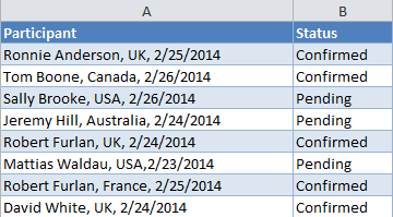
What we want is to separate data in one cell into several cells such as First Name, Last Name, Country, Arrival Date and Status. To have it done, perform the following steps:
- If you want to place the results in the middle of your table, start by inserting a new column(s) to avoid overwriting your existing data. In this example, we have inserted 3 new columns like shown in the screenshot below:
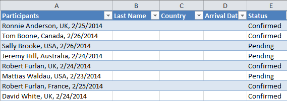
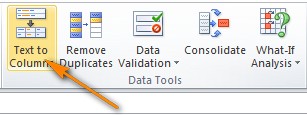
- Select the cells you want to divide, navigate to the Data tab > Data Tools group, and click the Text to Columns button.
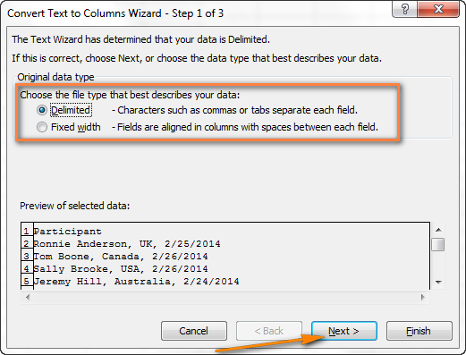
- In the first step of the Convert Text to Columns wizard, you choose how to split cells - by delimiter or width.In our case, the cell contents are separated with spaces and commas, so we select Delimited, and click Next.
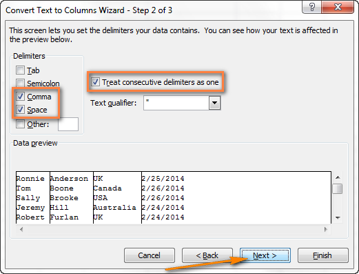
- In the next step, you specify the delimiters and, optionally, text qualifier.You can choose one or more predefined delimiters as well as type your own one in the Other box. In this example, we select Space and Comma:
Tips:
- Treat consecutive delimiters as one. Be sure to select this option when your data may contain two or more delimiters in a row, e.g. when there are a few consecutive spaces between words or the data is separate by a comma and a space, like "Smith, John".
- Specifying the text qualifier. Use this option when some text is enclosed in single or double quotes, and you'd like such portions of text to be inseparable. For example, if you choose a comma (,) as the delimiter and a quotation mark (") as the text qualifier, then any words enclosed in double quotes, e.g. "California, USA", will be put into one cell as California, USA. If you select {none} as the text qualifier, then "California will be distributed into one cell (together with an opening quotation mark) and USA" into another (together with a closing mark).
- Data preview. Before you click the Next button, it stands to reason to scroll through the Data preview section to make sure Excel has split all cells contents right.
- Just two more things are left for you to do - choose the data format and specify where you want to paste the resulting values:
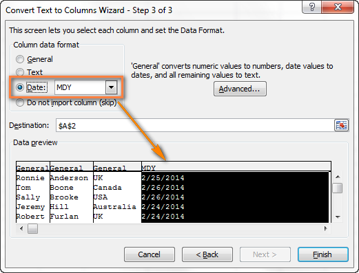
- Data format. By default, the General format is set for all columns, which works well in most cases. In our example, we need the Data format for the arrival dates. To change the data format for a particular column, click on that column under Data preview to select it, and then choose one of the formats under Column data format (please see the screenshot below).
- Destination. To tell Excel where you want to output the separated data, click the Collapse Dialog icon
 next to the Destination box and select the top-leftmost cell of the destination range, or type a cell reference directly in the box. Please be very careful with this option, and make sure there are enough empty columns right to the destination cell.
Notes:
- If you do not want to import some column that appears in the data preview, select that column and check Do not import column (skip) radio button under Column data format.
- It is not possible to import the split data to another spreadsheet or workbook. If you attempt to do this, you will get the invalid destination error.
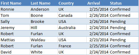
- Finally, click the Finish button and you are done! As shown in the below screenshot, Excel has perfectly placed the contents of one cell into several cells:
How to split text of a fixed width
This section explains how to divide a cell in Excel based on the number of characters you specify. To make things easier to understand, please consider the following example.
Supposing, you have Product IDs and Product names in one column and you want to extract the IDs into a separate column:
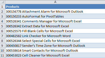
Since all of the product IDs contain 9 characters, the Fixed width option fits perfectly for the job:
- Start the Convert Text to Columns wizard as explained in the above example. In the first step of the wizard, choose Fixed width and click Next.
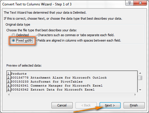
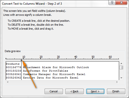
- Set the width of each column by using the Data preview section. As shown in the screenshot below, a vertical line represents a column break, and to create a new break line, you simply click at the desired position (9 characters in our case):
- In the next step, choose the data format and destination for the split cells exactly as we did in the previous example, and click the Finish button to complete the separation.
How to separate cells Excel with Flash Fill
Beginning with Excel 2013, you can make use of the Flash Fill feature that can not only automatically populate cells with data, but also split cell contents.
Let's take a column of data from our first example and see how Excel's Flash Fill can help us split a cell in half:
- Insert a new column next to the column with the original data and type the desired part of the text in the first cell (participant name in this example).
- Type the text in a couple more cells. As soon as Excel senses a pattern, it will populate similar data into other cells automatically. In our case, it's taken 3 cells for Excel to figure out a pattern:
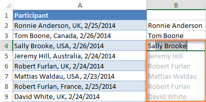
- If you are satisfied with what you see, press the Enter key, and all the names will be copied to a separate column at once.
How to split cell in Excel with formulas
Whatever diverse information your cells may contain, a formula to split a cell in Excel boils down to finding a position of the delimiter (comma, space, etc.) and extracting a substring before, after or in-between the delimiters. Generally, you'd use SEARCH or FIND functions to determine the delimiter's location and one of the Text functions (LEFT, RIGHT or MID) to get a substring.
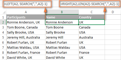
For example, you'd use the following formulas to split data in cell A2 separated with a comma and space (please see the screenshot below):
To extract the name in B2:
=LEFT(A2, SEARCH(",",A2)-1)
Here, the SEARCH function determines the position of a comma in A2, and you subtract 1 from the result, because the comma itself is not expected in the output. The LEFT function extracts that number of characters from the start of the string.
To extract the country in C2:
=RIGHT(A2, LEN(A2)-SEARCH(",", A2)-1)
Here, the LEN function calculates the total length of the string, from which you subtract the position of the comma returned by SEARCH. Additionally, you subtract the space character (-1). The difference goes to the 2nd argument RIGHT, so it pulls that many characters from the end of the string.
The result will look as follows:
If your delimiter is a comma with or without space, you can use the following formula to extract a substring after it (where 1000 is the maximum number of characters to pull):
=TRIM(MID(A2, SEARCH(",", A2)+1, 1000))
As you see, there is no universal formula that could handle all kinds of strings. In each particular case, you will have to work out your own solution.
The good news is that the dynamic array functions that appeared in Excel 365 make the use of many old formulas unnecessary. Instead, you can use these functions:
- TEXTSPLIT - split strings by any delimiter that you specify.
- TEXTBEFORE - extract text before a specific character or substring.
- TEXTAFTER - extract text after a certain character or word.
For more formula examples to divide cells in Excel, please check out the following resources:
Split cells using Split Text feature
Now that you are familiar with the inbuilt features, let me show you an alternative way to divide cells in Excel. I mean the Split Text tool included with our Ultimate Suite for Excel. It can perform the following operations:
- Split cell by character
- Split cell by string
- Split cell by mask (pattern)
For example, splitting the participant details in one cell into several cells can be done in 2 quick steps:
- Select the cells you want to separate, and click the Split Text icon on the Ablebits Data tab, in the Text group.
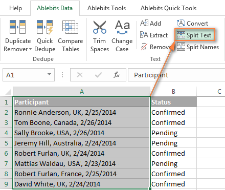
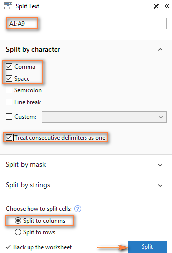
- On the add-in's pane, configure the following options:
- Select Comma and Space as the delimiters.
- Select the Treat consecutive delimiters as one check box.
- Choose Split to columns.
- Click the Split button.
Done! Four new columns with the split data are inserted between the original columns, and you only need to give those columns appropriate names:

Tip. To separate a column of names to the first name, last name and middle name, you can use a special Split Names tool.
If you are curious to see the Split Text and Split Names tools in action, we are welcome to use the download link below. I thank you for reading and hope to see you on our blog next week!
Available downloads
Ultimate Suite 14-day fully-functional version (.exe file)
 by
by
189 comments
Hi,
Could you help me to split the cells as written below to 4 MO and 500 FC ?
4 MO
OR
500 FC
Thanks
Hi! If I understand your task correctly, this guide may be helpful: Split string by line break. These formulas will be a complete solution to your problem.
Hi,
I have a data but I wanted to bring it out in the desired format.
How could I do it with shortcut?
Raw Data: Desired Format:
Dinner special 650 Dinner special 650
Cheez sting 120 Cheez sting 120
Cheez sting 120 Cheez sting 120
Lunch special 600 Lunch special 600
Thanks.
Hi! I am not sure I fully understand what you mean. What's the difference between Raw Data and Desired Format? Describe the problem in more detail.
Hi,
I have this data from Apple that I copied from my family's billing account.
The data is unfortunately in one column and each line is it's own cell.
I want to at least separate the left aligned data from the right aligned data.
It would be nice if I could also remove subsequent entries such as where it says discovery+ below.
However I can't just remove duplicates b/c there are many repeated entries that I need to retain...
Also to be noted that aside from the stated above; the transactions probably have some sort of trend, but are essentially random...
date
Transaction ID
Total $
discovery+
discovery+
discovery+ | Stream TV Shows
Renews Date
$$$$
Game BS
Game BS
Game
$$$$
Game BS
Game BS
Game
$$$$
Thanks!
Hi! An Excel formula can't determine whether the text in a cell is aligned right or left. I can't guess which cells you need. But you can use the FILTER function to get only the cells you need. For example, to get only the cells with the "$" symbol, the following formula would work:
=FILTER(A1:A25,ISNUMBER(SEARCH("$",A1:A25)))
To determine whether the desired character is in a cell, please read: How to find substring in Excel.
Well, comment entry field didn't like my formatting...
The "date" and "$$$$" is R aligned, everything else is L aligned.
Sorry for not clearly stating what I need (I am bad at conveying ideas to words).
However if possible, I simply want to move/separate the date, transaction ID, $$ and description/titles.
Your description is not quite clear. Describe exactly what result you want to get from your data.
Hi, i have a problem, is there a formula to split names that is in one column seperated by comma and space. I want it to split into one column but, every other text in new row, and if is possible to count how many times specific name repeates in column.
Original
Column 1
Bernard Bezjak, Laura Krajnc, Petra Miško, Mateja Krajnc
-----------------------------------------------------------------------------------
Bernard Bezjak, Laura Krajnc, Mateja Krajnc
Result
Column 1 Column 2
Bernard Bezjak 2
Laura Krajnc 2
Petra Miško 1
Mateja Krajnc 2
Hi! Get a list of unique values from the text strings in column A using the formula
=UNIQUE(TEXTSPLIT(TEXTJOIN(", ",,A1:A20),,", "))
If this formula is written, for example, in cell E1, then you can count how many times a specific name repeated in column using the formula
=SUM(--(TEXTSPLIT(TEXTJOIN(", ",,$A$1:$A$2),,", ")=E1))
For more information, read: TEXTSPLIT function in Excel: split text strings by delimiter, Excel UNIQUE function - fastest way to find unique values.
Hi!
If I need help breaking information down, for example, 300ABNMCT4-150
I need the information to be displayed as below:
(Cell1) 300A
(Cell2) BN
(Cell3) MC
(Cell4) T4
(Cell5) -
(Cell6) 150
Any ideas please?
Many thanks!
Hi! Your text string has no delimiters with which to split it the way you want. So use the MID function to get each part of the text.
Hi could you please help me in this example: data which I need to split is in a text file and like this:
Shivani, marketing field, 42,green avenue
143001, amritsar
Shivam, it field, 37, lohgarh gate
143001, amritsar
I want to convert it into:
Shivani | marketing field| 42,green avenue|143001 | amritsar
Shivam |it field | 37, lohgarh gate| 143001 |amritsar
Hi!
You cannot use a comma as a separator because it is used inside the address. Therefore, you cannot automatically separate text the way you want to do it.
Name1 Name2 Name3 Name4 Name5 Name6
How split every name by space in columns
Col1 Col2 Col3 Col4 Col5 Col6
Name1 Name2 Name3 Name4 Name5 Name6
Please help
Hi!
Try to read the article above carefully.
=LEFT(A1, SEARCH(".",A1)-1) was a starting point and helpful for me, I am interested in the next part if possible, see below text string
27/10/22 08:34 Email sent to applicant asking them to complete their online form (xxxx.co.uk). 27/10/22 08:34 Sent SMS to the applicant asking them to complete their application form (xxxx). 27/10/22 08:34 Client has added this guarantor from within their login area. 27/10/22 12:49 Application form received and reference moved to 'Waiting Approval' status. 27/10/22 12:49 Credit checks completed for xxxxxx 27/10/22 14:19 Client has elected to go ahead with this reference at the Waiting Approval stage.
If the above is all in one cell how would I separate them into columns starting with the date
Hi!
To split a cell, define delimiters in your text as described in the article above.
Hi Guys,
I'm hoping you might be able to point me in the right direction of splitting something like this:
Column1 Column2
Row1 #1 Part1, Part2, Part3
Row2 #2 Part1, Part4
Row3 #3 Part3, Part5, Part6
Into something like this (if it's possible):
Column1 Column2
Row1 #1 Part1
Row2 #1 Part2
Row3 #1 Part3
Row4 #2 Part1
Row5 #2 Part4
Row2 #3 Part3
Row1 #3 Part5
Row2 #3 Part6
Any help will be greatly appreciated! Cheers!
Hi!
Try to follow the recommendations from this article: TRANSPOSE function in Excel: rotate columns to rows.
Thanks Alexander,
Your comment helped lead me down the rabbit hole all the way to the "Power Query" feature which did the trick.
Cheers mate!
1236(21)_1429(5710) = 1236 | 21 | 1426 | 570
2447(28). = 2447 | 28
1(631). = 1 | 631
How can split these numbers " 1236(21)_1429(5710) " into deferent colums?
Hello!
Apply the methods described in the article above using 3 different delimiters: "(", ")" and "_".
Also, you can use the formulas recommended in this guide: How to split text string in Excel by comma, space, character or mask. Since you have 3 delimiters, the formula or other method needs to be applied 3 times with each delimiter.
How to make the delimiter be aligned at the same position in all rows
Hi i need a formula to slipt the text and number.
e.g.
he is looking for 50.
he is looking for a guy who is earning 1000 but should not be disable.
100 required to book a hotel. etc.
Hi!
The following tutorial should help: How to extract number from text string.
Hello!!!
I have a situation where I need to count letter after a different letter in a range.
For Eg:
1 2 3 4 5 6 7 8 9
A P P P P A P P P
I need only "P" letter to be counted after letter "A" is the condition. So, the result should be 3.
Please let me know the formula to get the result.
Thank you in advance!!!
Dear All, I need code to split this: 0.50, 0.67, 0.83 into different columns. Thank you.
Hi!
Have you tried the ways described in this blog post? Why couldn't you use them?
Container No
BMOU4616547(45G1), CXDU1285280(22G1), UETU2524349(20G1), CSNU1222152(22G0), OOLU1592935 (25G0), TRHU3872670(20G0), CSNU6027170(45G0)
Dear sir/madam
Above data is included in one Colum, i want only last code to separate the data.
how to split (45G1,22G1,20G1,22G0,25G0,45G0) In separate Colum.
please advise the same
Hi!
I'd recommend you to have a look at Split text tool.
It can split delimited text into columns. Use a mask
*(*)*
It is available as a part of our Ultimate Suite for Excel that you can install in a trial mode and check how it works for free.
Hi I have a column which contains three formats of data.
I need to sepearate the last three letters from the rest of the number (e.g. 1)/ number and letter (e.g. 2).
I tried text to column, but as there is no space or comma to spearte the stuff out, how can I separate it?
E.g.
1. 598284CAV
2. H28597KAL
Thanks in advance.
Shraddha
Hello!
You can separate the last 3 characters from the text using the RIGHT function.
I hope I answered your question.
Strauss Needle Diamond Bur Medium-E11M
Strauss Needle Diamond Bur Medium E31M
Strauss Flat End Cylinder Medium-D32M
Strauss Precision Depth Marker Red AD15C
Strauss Barrel Diamond Bur Coarse-M4C
Strauss Flat End Cylinder Coarse-D31C
Want to know how to separate codes from text
Hello!
Here is the formula that should work perfectly for you:
=TRIM(RIGHT(SUBSTITUTE(TRIM(RIGHT(SUBSTITUTE(A1,"-",REPT(" ",20)),20))," ",REPT(" ",20)),20))
I hope I answered your question. If something is still unclear, please feel free to ask.
This formula is amazing!!! Thank you so much for sharing. It has saved me and my team so much time and extra work.
Hello, I have a question. How do I separate if the delimiters are not consistent in the column?
Ex:
aaaaa_bbbbb
aaaaa-bbbbb
aaaaa_bbbbb
aaaaa-bbbbb
some use "_" while others use "-"
Hope someone can help me.
Thanks
Hello!
We have a tool that can solve your task in a couple of clicks - Ablebits Data - Split text.
It is available as a part of our Ultimate Suite for Excel that you can install in a trial mode and check how it works for free
How to prepare a dynamic sheet in excel with values in below sequence, but not of equal length but break from "-".
AB-CDEF-GHI-JK-LMN
A-BCDEF-G-HIJ-LMNO
This is the sequence of data.
con you please guide me to create a dynamic formulae -having output reads as below.
"AB" "CDEF" "GHI" "JK" "LMN"
Hello!
Please read the above article carefully.
Hi,
How can I split the following information by slash:
WMCF1GL0621Z\TVIPACKBM1\WaferMapRecipe
Col A1: WMCF1GL0621Z
Col B1: TVIPACKBM1
Col C1: WaferMapRecipe
Thanks in advacne.