The tutorial shows how to do subtraction in Excel by using the minus sign and SUM function. You will also learn how to subtract cells, entire columns, matrices and lists.
Subtraction is one of the four basic arithmetic operations, and every primary school pupil knows that to subtract one number from another you use the minus sign. This good old method works in Excel too. What kind of things can you subtract in your worksheets? Just any things: numbers, percentages, days, months, hours, minutes and seconds. You can even subtract matrices, text strings and lists. Now, let's take a look at how you can do all this.
Subtraction formula in Excel (minus formula)
For the sake of clarity, the SUBTRACT function in Excel does not exist. To perform a simple subtraction operation, you use the minus sign (-).
The basic Excel subtraction formula is as simple as this:
For example, to subtract 10 from 100, write the below equation and get 90 as the result:
=100-10
To enter the formula in your worksheet, do the following:
- In a cell where you want the result to appear, type the equality sign (=).
- Type the first number followed by the minus sign followed by the second number.
- Complete the formula by pressing the Enter key.
Like in math, you can perform more than one arithmetic operation within a single formula.
For example, to subtract a few numbers from 100, type all those numbers separated by a minus sign:
=100-10-20-30
To indicate which part of the formula should be calculated first, use parentheses. For example:
=(100-10)/(80-20)
The screenshot below shows a few more formulas to subtract numbers in Excel:

How to subtract cells in Excel
To subtract one cell from another, you also use the minus formula but supply cell references instead of actual numbers:
For example, to subtract the number in B2 from the number in A2, use this formula:
=A2-B2
You do not necessarily have to type cell references manually, you can quickly add them to the formula by selecting the corresponding cells. Here's how:
- In the cell where you want to output the difference, type the equals sign (=) to begin your formula.
- Click on the cell containing a minuend (a number from which another number is to be subtracted). Its reference will be added to the formula automatically (A2).
- Type a minus sign (-).
- Click on the cell containing a subtrahend (a number to be subtracted) to add its reference to the formula (B2).
- Press the Enter key to complete your formula.
And you will have a result similar to this:

How to subtract multiple cells from one cell in Excel
To subtract multiple cells from the same cell, you can use any of the following methods.
Method 1. Minus sign
Simply type several cell references separated by a minus sign like we did when subtracting multiple numbers.
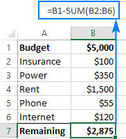
For example, to subtract cells B2:B6 from B1, construct a formula in this way:
=B1-B2-B3-B4-B5-B6

Method 2. SUM function
To make your formula more compact, add up the subtrahends (B2:B6) using the SUM function, and then subtract the sum from the minuend (B1):
=B1-SUM(B2:B6)
Method 3. Sum negative numbers
As you may remember from a math course, subtracting a negative number is the same as adding it. So, make all the numbers you want to subtract negative (for this, simply type a minus sign before a number), and then use the SUM function to add up the negative numbers:
=SUM(B1:B6)

How to subtract columns in Excel
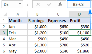
To subtract 2 columns row-by-row, write a minus formula for the topmost cell, and then drag the fill handle or double-click the plus sign to copy the formula to the entire column.
As an example, let's subtract numbers in column C from the numbers in column B, beginning with row 2:
=B2-C2

Due to the use of relative cell references, the formula will adjust properly for each row:
Subtract the same number from a column of numbers
To subtract one number from a range of cells, enter that number in some cell (F1 in this example), and subtract cell F1 from the first cell in the range:
=B2-$F$1
The key point is to lock the reference for the cell to be subtracted with the $ sign. This creates an absolute cell reference that does not change no matter where the formula is copied. The first reference (B2) is not locked, so it changes for each row.
As the result, in cell C3 you will have the formula =B3-$F$1; in cell C4 the formula will change to =B4-$F$1, and so on:

If the design of your worksheet does not allow for an extra cell to accommodate the number to be subtracted, nothing prevents you from hardcoding it directly in the formula:
=B2-150
How to subtract percentage in Excel
If you want to simply subtract one percentage from another, the already familiar minus formula will work a treat. For example:
=100%-30%
Or, you can enter the percentages in individual cells and subtract those cells:
=A2-B2

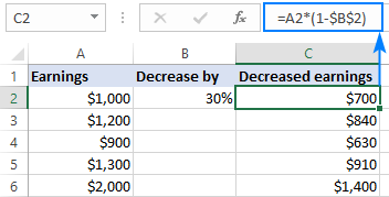
If you wish to subtract percentage from a number, i.e. decrease number by percentage, then use this formula:
For example, here's how you can reduce the number in A2 by 30%:
=A2*(1-30%)
Or you can enter the percentage in an individual cell (say, B2) and refer to that cell by using an absolute reference:
=A2*(1-$B$2)
For more information, please see How to calculate percentage in Excel.
How to subtract dates in Excel
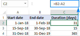
The easiest way to subtract dates in Excel is to enter them in individual cells, and subtract one cell from the other:
You can also supply dates directly in your formula with the help of the DATE or DATEVALUE function. For example:
=DATE(2018,2,1)-DATE(2018,1,1)
=DATEVALUE("2/1/2018")-DATEVALUE("1/1/2018")
More information about subtracting dates can be found here:
How to subtract time in Excel
The formula for subtracting time in Excel is built in a similar way:
For example, to get the difference between the times in A2 and B2, use this formula:
=A2-B2
For the result to display correctly, be sure to apply the Time format to the formula cell:
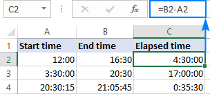
You can achieve the same result by supplying the time values directly in the formula. For Excel to understand the times correctly, use the TIMEVALUE function:
=TIMEVALUE("4:30 PM")-TIMEVALUE("12:00 PM")
For more information about subtracting times, please see:
How to do matrix subtraction in Excel
Suppose you have two sets of values (matrices) and you want to subtract the corresponding elements of the sets like shown in the screenshot below:
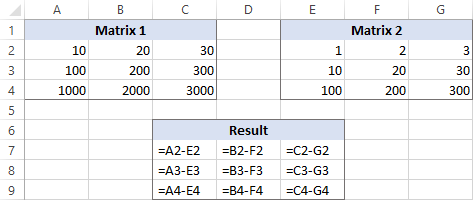
Here's how you can do this with a single formula:
- Select a range of empty cells that has the same number of rows and columns as your matrices.
- In the selected range or in the formula bar, type the matrix subtraction formula:
=(A2:C4)-(E2:G4) - Press Ctrl + Shift + Enter to make it an array formula.

The results of the subtraction will appear in the selected range. If you click on any cell in the resulting array and look at the formula bar, you will see that the formula is surrounded by {curly braces}, which is a visual indication of array formulas in Excel:
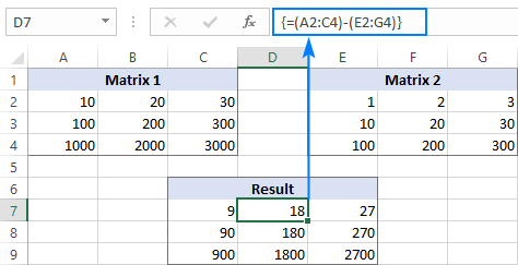
If you do not like using array formulas in your worksheets, then you can insert a normal subtraction formula in the top leftmost cell and copy in rightwards and downwards to as many cells as your matrices have rows and columns.
In this example, we could put the below formula in C7 and drag it to the next 2 columns and 2 rows:
=A2-C4
Due to the use of relative cell references (without the $ sign), the formula will adjust based on a relative position of the column and row where it is copied:

Subtract text of one cell from another cell
Depending on whether you want to treat the uppercase and lowercase characters as the same or different, use one of the following formulas.
Case-sensitive formula to subtract text
To subtract text of one cell from the text in another cell, use the SUBSTITUTE function to replace the text to be subtracted with an empty string, and then TRIM extra spaces:
With the full text in A2 and substring you want to remove in B2, the formula goes as follows:
=TRIM(SUBSTITUTE(A2,B2,""))
As you can see, the formula works beautifully for subtracting a substring from the beginning and from the end of a string:

If you want to subtract the same text from a range of cells, you can "hard-code" that text in your formula.
As an example, let's remove the word "Apples" from cell A2:
=TRIM(SUBSTITUTE(A2,"Apples",""))

For the formula to work, please be sure to type the text exactly, including the character case.
Case-insensitive formula to subtract text
This formula is based on the same approach - replacing the text to subtract with an empty string. But this time, we will be using the REPLACE function in combination with two other functions that determine where to start and how many characters to replace:
- The SEARCH function returns the position of the first character to subtract within the original string, ignoring text case. This number goes to the start_num argument of the REPLACE function.
- The LEN function finds the length of a substring that should be removed. This number goes to the num_chars argument of REPLACE.
The complete formula looks as follows:
Applied to our sample data set, it takes the following shape:
=TRIM(REPLACE(A2,SEARCH(B2,A2),LEN(B2),""))
Where A2 is the original text and B2 is the substring to be removed.

Subtract one list from another
Supposing, you have two lists of text values in different columns, a smaller list being a subset of a larger list. The question is: How do you remove elements of the smaller list from the larger list?
Mathematically, the task boils down to subtracting the smaller list from the larger list:
Larger list: {"A", "B", "C", "D"}
Smaller list: {"A", "C"}
Result: {"B", "D"}
In terms of Excel, we need to compare two lists for unique values, i.e. find the values that appear only in the larger list. For this, use the formula explained in How to compare two columns for differences:
=IF(COUNTIF($B:$B, $A2)=0, "Unique", "")
Where A2 is the first cells of the larger list and B is the column accommodating the smaller list.
As the result, the unique values in the larger list are labeled accordingly:
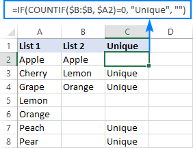
And now, you can filter the unique values and copy them wherever you want.
That's how you subtract numbers and cells in Excel. To have a closer look at our examples, please feel free to download our sample workbook below. I thank you for reading and hope to see you on our blog next week!
Practice workbook
Subtraction formula examples (.xlsx file)
 by
by
110 comments
how can i subtract row into excel sheet , when trying to reconcile a data.
eg, data are cash book statement and bank statement as which they are identical into transaction of control number but some times amount being different as per as same control number.
control number amount
995810468084 15,000.00
995810468084 15,000.00
995810468085 15,000.00
995810468085 15,000.00
995810468086 26,800.00
995810468086 26,800.00
995810468087 15,000.00
995810468087 15,000.00
995810468088 63,500.00
995810468088 63,500.00
Hi! I’m not sure I got you right since the description you provided is not entirely clear. However, it seems to me that the formula below will work for you:
=SUMIF($A$2:$A$10,A2,$B$2:$B$10)/2=B2
This formula returns TRUE if the amounts for the same control numbers match, and returns FALSE if they do not match. For more information, please visit: How to use SUMIF function in Excel with formula examples.
I have a weekly timecard and F2 totals 40 hrs G2 is Overtime hrs and i want G2 to autofilll
The total hours over 40 automatically … in OT column, leaving the 40 in F2,
Would i use :
=sum d2-c2 <40 ?
Ie: Tot OT
A2 B2 C2 D2 E2 F2 G2
8. 8. 8. 8. 9. 40. 1
8. 8. 8. 8. 7 39. 0
Hello Debbi!
If I understand your question correctly, the SUM function is being used to calculate the total number of worked hours. For example:
=SUM(A2:E2)-F2
I’m trying to subtract cells A1 through A10, how do I do that without having to list each cell separately?
Hello Dana!
If I understand your question correctly, you can use the SUM function to subtract all cells A1 through A10 at once.
=B1-SUM(A1:A10)
Hi - How can i show a 'negative value' in the formula =SUM(X15-X17) where cell X17 is more than cell X15 - i.e. 2 - 3 = -1 - & how do i show this in red font / colour - thanks
Hello Mac!
You can change font color with custom number format. To show a negative value in red, you can use such a custom number format:
0.00;[Red]-0.00
I recommend reading this guide: Custom Excel number format.
Good morning, I am trying to subtract E2-D2 into F2 with the answer also populating on the next row of E2. I want to be able to subtract an expense while tracking what money is left.
Hi! You cannot use one formula to write values to E3 and F2. Use a separate formula for each cell. Maybe this article will be helpful: Excel Cumulative Sum - easy way to calculate running total.
Hi, i was asked to create a spreadsheet that shows the quantity of items, how much was issued out, when it was issued out and what's remaining plus for it to be continuous? and to make a formula that allows the other person to just put in the info numbers.
How do i go about this?
Hi! I won't be able to create a spreadsheet for you with data that I don't have. If you have a specific question about how to calculate a value or create a formula, please ask me.
I am wanting to enter a total dollar amount subtracted by dollar amount spent that I enter and then the formula to calculate the total remaining balance by percentage total instead of a dollar amount total. Help....
Example
Column A Column B Column C
$1000 $230 23%
Hi! Look for the example formulas here: How to calculate percentage in Excel.
I was looking to see if there was a formula that I can use to subtract letters used in a cell from a specific number. For example:
If I had the number 33 in a cell which accounts for 33 days annual leave, and I used the letters H (holiday) and BH (bank holiday).
What formula can I use that would subtract a number from the 33 whenever an H or BH is entered.
If I start with the 33 and use 5 days holiday and entered H five times on a spreadsheet, the 33 would automatically come down to 28.
I hope this makes sense. Thanks
Hi! If you enter the letter "H" in a certain range of cells, you can use the COUNTIF function to count the number of such letters. Subtract the resulting number from the cell containing the number 33. For example:
=A1-COUNTIF(B1:Z1,"H")
I recommend reading this guide: COUNTIF function in Excel - count if not blank, greater than, duplicate or unique.
I am working on a monthly budget sheet where I am listing all dollar amounts into one column (H). H2 shows the amount of monthly income to start out with, H5 lists the amount of the first bill. H6 is a subtotal line where I would enter the following: =SUM(H2-H5). H7 is the next bill, H8 is a subtotal line where I would enter the following: =SUM(H6-H7), etc., etc.
Is there a formula for doing this automatically, or is adding the =SUM(H-H) in every subtotal row and final total row the only way?
Hi! Autofill in Excel only works for consecutive cells that follow each other. This is not the case in your situation.
Teach me more
I want to subtract 2 filtered rows having 4 coloumns. and i want to keep the subtraction action as is. Whenever i change the filtered criterions, the formula should apply automatically again and sow the result. Something similar to subtotal function, but i want it for subtraction function. how can i do it?
Is there a formula where we can continually subtract an amount from a number until the initial number is less than the subtracted number and stop?
Example: 94831 - 10000 but answer will show 4831.
I would like to know if there is a way to set up a formula in Excel spreadsheet whereby each week the number in the cell/column reduces by 1 = eg 42 -1 = 41 - 1 =40 and so on every time you open the spreadsheet?
Hi! See answer to a similar question in this comment.
Hi, I have a question. If I want to take the number from sheet 2(e.g. B13), and use it in the sheet 1, I start to type
='sheet 2'!B13
in sheet 1,
What if I want the number in sheet 2(from C2 to H7), (in a diagonal way), should I type
='sheet 2'!C2
='sheet 2'!COLUMN(C+1),ROW(2+1)
='sheet 2'!COLUMN(C+2),ROW(2+2)
='sheet 2'!COLUMN(C+3),ROW(2+3)
='sheet 2'!COLUMN(C+4),ROW(2+4)
='sheet 2'!COLUMN(C+5),ROW(2+5)
instead of
='sheet 2'!C2
='sheet 2'!D3
='sheet 2'!E4
='sheet 2'!F5
='sheet 2'!G6
='sheet 2'!H7
I know I am wrong, and I want a faster way to deal with the data.😭
EXTRA QUESTION......
What if one of the data from C2 to H7 is 0(zero), how can it automatically skip it and jump to the next one?🤔
Hi,
I want a formula to calculate and find the difference between two different rows and columns, For eg, assume cells from rows B5:E5 is 4 and column F1:F4 is 4. now i want to calculate and find the difference between these on F5 and the result should be 0 on F5. Can you suggest a formula?
What formula
Would I use to subtract the quantity of items sold column from the quantity items in stock column. For example: quantity available is 5. Quantity sold is 3. Which formula would I use to make the quantity available column change to 2?
The available quantity is the difference between the purchased goods and the sold goods.
Hi!
To calculate the difference between the ranges, I suggest using the SUM function:
=SUM(B5:E5)-SUM(F1:F4)
or
=SUM(B5:E5-F1:F4)
A1 indicates the number of community service hours, if the community service hour goal of 500 hours was met. Create a function that will identify if the goal was achieved
Hi!
For conditional calculations, use the IF function.
Create a formula that will subtract the value of D1 which is 22 from the value of A1 which is 12.
Hi!
The answer is in the first paragraph of this article.
How do you write a formula in excel which compares 4 numbers in 4 particular cells in order to determine the lowest number. Then subtract this lowest number from itself to arrive at 0 and also from the other 3 numbers in the 3 other cells to arrive at a new number.
Say the lowest number of the 4 numbers was 8 and the other 3 numbers were 12, 16 & 20. Then when a formula is inserted to compare those numbers the answers would automatically be 0, 4, 8 & 12.
Hello!
To find the minimum number in a range, use the MIN function:
=(A1:A4)-MIN(A1:A4)
Okay thanks
Hello,
I am working on an employee timesheet where they inform the hours worked and if they were OFF.
The formula is simple to see the hours worked, but I am struggling with the text (OFF) as I am getting the #VALUE! error.
Example: Start(C4) 8:00 / Finish (D4) 12:00 / Break(E4) 0:30 = (Finish - Start - Break)*24 = 3.50h
My problem is when they are OFF part time or full time. I have found the formula below that worked when they are all day OFF = showing 0h. But doesn't work when they inform hours.
=IF(ISERROR(D4*1),0,D4)-IF(ISERROR(C4*1),0,C4-IF(ISERROR(E4*1),0,E4))*24
Any help will be great, thank you in advance.
KR,
Graziella
Hi!
If "off" is written in cell D4, then you get a negative time, which is impossible. If there is a start time, then there must be an end time.
Thank you Alexander. Yes we always have the 3 information : start, finish and break. Is there any formula that understand the text as ZERO so and work correctly when there are hours as well?
Right now I do manually but really want to find something more easier.
Hi!
Your formula will convert text to zero. But if you write the end time "off", you will always get an error. You will subtract the start time from zero. I don't understand how the end time can be "off". What result do you want to get? Give an example of the source data and the expected result.
I also recommend reading this article: Calculate time in Excel: time difference, add, subtract and sum times.
Hello,
I've been trying to work this out for a while. So for example I want to 100-10, which equal 90. Then from that 90 get 40% which is 36. This should then be 54. However, I cannot seem to find a formula that works for me.
Thanks in advance!
Hi!
It's just simple math. =(100-10)*40%. or (100-10)*(100%-40%). Your explanations are not very clear. The following tutorial should help: How to do calculations in Excel.
Sorry! And thank you for that!
How to calculate (A%-B%) in excal