Today, we are going to do Vlookup in Excel with several different formulas, measure their calculation speed and evaluate consistency, so you can choose your winner.
Finding information across different tables is one of the most common tasks in Excel. Regrettably, the classic VLOOKUP function is notorious when it comes to processing power and flexibility. It's no wonder that over the years Excel users have come up with their own solutions such as an INDEX MATCH formula. Luckily, Microsoft has finally realized that VLOOKUP has too many weaknesses and released a more powerful successor - the XLOOKUP function. So, which one is the best to use?
If your tables have only a few dozen rows, then most likely any method will be quick enough, and you won't notice the difference. But if the number of rows is measured in thousands, the correct choice of the function is crucial - the difference in performance can be more than 10 times! So, let's start the timer and see who is the fastest :)
Source data
In all the examples, we well be using the following data set:
- Main table containing 500,000 rows
- Lookup table containing 500 rows
Our goal is to match the items names and pull the prices from the lookup table into the main table.
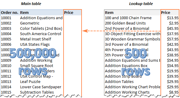
For each method, we will enter the formula in C2 and copy it down through C500001, measuring the time it takes Excel to calculate half a million cells.
Naturally, the result will depend on many factors such as your CPU performance, RAM size, Excel version, etc. In this experiment, it is not absolute numbers that matter. It's more important to understand the performance of each formula in comparison, their advantages and drawbacks.
Our examples assume that you have the basic knowledge of the functions, and we won't dwell much on their syntax. Links to in-depth tutorials are included for your convenience.
All tests were carried out on my Dell laptop (Intel Core i5-8250U; RAM 16 GB) with Microsoft 365 Apps for business installed; Excel 32-bit, version 2011, build 13415, Beta Channel. The same tests were also performed by my colleague on Excel 64-bit, and some results are drastically different!
VLOOKUP formula
When it comes to looking up and retrieving matching data in Excel, the first function that comes to mind is the good old VLOOKUP. In fact, it's not that good as it could be, but we'll talk this a bit later :)
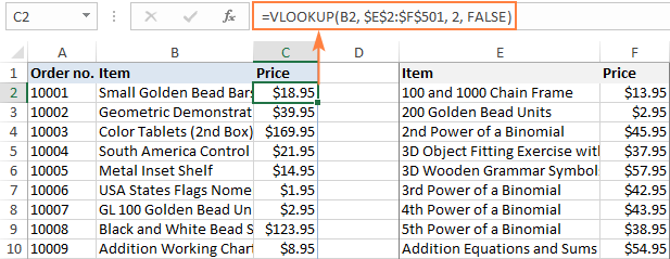
To pull prices from the lookup table (E2:F501) to the main table (A2:B500001), we define the following arguments for our VLOOKUP formula:
- Lookup_value: B2 - the value to search for in the lookup table.
- Table_array: $E$3:$F$501 - please notice that we lock the references with the $ sign so that they don't shift when copying the formula.
- Col_index_num: 2 - the data is to be retrieved from the 2nd column of the lookup table.
- Range_lookup: FALSE - looking up for exact match.
The complete formula is:
=VLOOKUP(B2, $E$3:$F$501, 2, FALSE)
The above formula goes to C2, and then we double click the plus sign in the lower right corner to copy the formula across the entire column. At the moment of double-clicking, we run a stopwatch and see that this calculation takes 6.6 seconds.
When doing Vlookup in real worksheets, many people supply the entire columns for table_array to cater for possible additions in the future:
=VLOOKUP(B2, E:F, 2, FALSE)
Does it affect the performance? Yes, it does. It takes 14.2 seconds to calculate the entire column. That was hard to believe, so I double checked. The same result - less than half the speed of the ranges.
Apart from being swift, your formula also needs to be robust and durable, right? Regrettably, VLOOKUP cannot boast of reliability and resilience.
VLOOKUP limitations
As already mentioned, Excel VLOOKUP has a number of irritating constraints. The most essential ones are:
- Cannot look at its left. The VLOOKUP function can only look in the leftmost column of the table array and return information from the right.
- Does not survive the column insertion or deletion. Because the return column is specified as an index number, a VLOOKUP formula stops working as soon as a new column is added to or removed from the table array.
- A lookup value is limited to 255 characters.
Calculation time: range - 6.6 seconds; entire columns - 14.2 seconds.
In-depth tutorial: Excel VLOOKUP examples for beginners
INDEX MATCH formula
For many users, an advanced form of lookup in Excel is the magical INDEX MATCH formula. In generic form, it looks like this:
For our data set, the formula takes this form:
=INDEX($F$2:$F$501, MATCH(B2, $E$2:$E$501, 0))
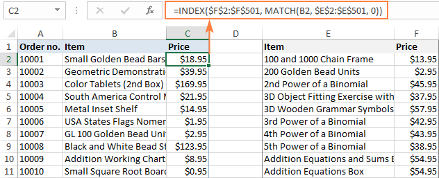
As with VLOOKUP, please remember to use absolute references for lookup and return ranges to ensure that the formula copies correctly to the below cells.
With both tables on the same sheet, INDEX MATCH performed much slower than VLOOKUP (8.9 against 6.6 seconds).
But if we move the lookup table to another worksheet, the formula starts working much faster (~ 5 seconds), which is better than VLOOKUP.
Anyway, INDEX MATCH makes up the time with a number of vital benefits.
INDEX MATCH advantages
- Can look from right to left. Yep, an INDEX MATCH formula does not care where the lookup column is located, because unlike VLOOKUP it explicitly defines a lookup range rather than a table array.
- Immune to column insertion and deletion. With INDEX MATCH, you can add and remove columns safely since you specify a return range, not an index number.
- No limit for a lookup value's size. While VLOOKUP is limited to 255 characters, INDEX MATCH has no problems with processing longer strings.
- Can perform Vlookup with multiple criteria as shown in the above linked example.
- Can do a 2-dimensional lookup and return a value at the intersection of a specific row and column.
Calculation time: ranges - 8.9 seconds; entire columns - 17.7 seconds; from another sheet - 5.2 seconds.
In-depth tutorial: INDEX MATCH formula in Excel
OFFSET MATCH formula
Here is one more formula to look up vertically in Excel, which is free of many limitations of VLOOKUP:
Where:
- n - is the lookup column offset that specifies how many columns to move from the beginning of the table to the lookup column.
- m - is the return column offset that determines how many columns to move to the return column.
In our case, the lookup column offset (n) is 0 because we are searching in the first column, so no shift is needed. The return column offset (m) is 1 because the matches are in the second column, and we need to move 1 column to the right to get to them:
=OFFSET($E$2:$F$501, MATCH(B2, OFFSET($E$2:$F$501, 0, 0, ROWS($E$2:$F$501), 1), 0) -1, 1, 1, 1)
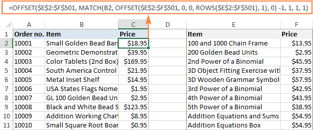
Compared to the previous solutions, the formula is too cumbersome, right? However, it is much faster than VLOOKUP or INDEX MATCH. Calculating 500 thousand rows takes less than 3 seconds! On entire columns, OFFSET is just a little slower - 3.5 seconds.
=OFFSET(E:F, MATCH(B2, OFFSET(E:F, 0, 0, ROWS(E:F), 1), 0) -1, 1, 1, 1)
In Excel 64-bit, however, the result is not so impressive - around 7.5 seconds. Why's that? A good question to Microsoft guys :)
OFFSET MATCH advantages
Aside from speed, this formula has a few other merits:
- Can perform a right-to-left Vlookup and upper Hlookup.
- Can do a two-way lookup based on the column and row values.
- Does not break when columns are inserted in or deleted from the lookup table.
OFFSET MATCH drawback
Complex syntax.
Calculation time: ranges - 2.9 seconds; entire columns - 3.5 seconds.
In-depth tutorials:
XLOOKUP formula
Microsoft 365 subscribers are provided with a new and more powerful function to look up information in their worksheets:
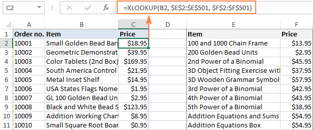
For our purpose, the defaults of the last 3 arguments work just fine, so we specify only the first 3 parameters, which are required. The arguments' names are intuitive, and I believe you can understand the formula without additional explanations:
=XLOOKUP(B2, $E$2:$E$501, $F$2:$F$501)
XLOOKUP advantages
Compared to traditional VLOOKUP, the XLOOKUP function has many improvements such as:
- Simplified and more meaningful syntax
- Ability to look up vertically and horizontally in any direction: right, left, bottom or up.
- For sorted data, it has a special binary search mode that is a lot faster than regular search.
- Search in reverse order to get the last occurrence.
- Ability to return multiple values.
- Handle more than one condition as explained in Excel XLOOKUP with multiple criteria.
- Inbuilt If error functionality.
XLOOKUP drawbacks
XLOOKUP is only available in Excel 365 and 2021. In Excel 2019, Excel 2016 and earlier versions, it is not supported.
And now, let's see how speedy this new function is. 11.2 seconds - quite disappointing :(
What if we use column references instead of ranges?
=XLOOKUP(B2, E:E, F:F)
24.5 seconds. No words… Nearly twice as slow as VLOOKUP.
Calculation time: ranges - 11.2 seconds; entire columns - 24.1 seconds.
Comprehensive tutorial: Excel XLOOKUP function with examples
Vlookup in Excel tables
As you probably know, data in Excel tables can be referenced in a special way - by using table and column names instead of cell addresses. This is called a structured reference, and I wonder if it has any impact on the calculation speed.
To check this, let's convert ranges to tables and re-test our formulas.
For convenience, our tables are named Main_table (A1:C500001) and Lookup_table (E1:F5001).
To create a table reference, start typing the formula in the first cell (C2), select the cells and ranges you want to refer to, and Excel will insert the structured references automatically.
For example, here's how the VLOOKUP formula looks like:
=VLOOKUP([@Item], Lookup_table, 2, FALSE)
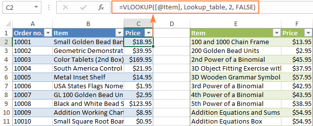
A great feature of Excel tables is that as soon as you enter a formula in just one cell, it is immediately populated in all other cells in the same column. Besides, tables are dynamic by nature and expand automatically to include any new data that you type next to a table.
In our table, the VLOOKUP formula calculated in 2.3 seconds, INDEX MATCH in 2.6 seconds, OFFSET and MATCH in 2.7 seconds, and XLOOKUP in 3.3 seconds. As you see, the calculation speed increases significantly compared to ranges.
The formulas are listed below for your reference:
=INDEX(Lookup_table[Price], MATCH([@Item], Lookup_table[Item], 0))
=OFFSET(Lookup_table, MATCH([@Item], OFFSET(Lookup_table, 0, 0, ROWS(Lookup_table), 1), 0) -1, 1, 1, 1)
=XLOOKUP([@Item], Lookup_table[Item], Lookup_table[Price])
Interestingly enough, Excel tables are very fast even with regular references. That is, if you convert only the first range (A1:C500001) to a table and use a normal VLOOKUP formula to pull data from the lookup range, the entire column in the main table will get calculated in about 2.5 seconds!
Calculation speed: from 2.3 to 3.3 seconds depending on the formula.
End-to-end tutorials:
Vlookup with dynamic arrays
The groundbreaking change in the Excel 365 calculation engine that occurred in January 2020 has added support for the so-called dynamic arrays. In short, these are resizable arrays that calculate automatically and return values into multiple cells based on a formula entered in one cell.
One of the best things about dynamic arrays is that they can be used with almost any traditional Excel function. For our VLOOKUP formula, it will look like this:
=VLOOKUP(B2:B500001, E2:F500001, 2, FALSE)
The difference with the classic VLOOKUP function is that you supply the entire lookup array for the first argument, not a single lookup value. Because the formula is entered just in one cell, you needn't worry about locking the ranges with absolute references.
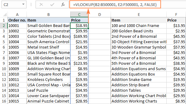
As for performance, dynamic arrays work even faster than Excel tables! Half a million cells are filled with the results almost immediately: 1.8 seconds - very impressive!
Other results are listed below:
INDEX MATCH - 4.4 seconds
=INDEX(F2:F501, MATCH(B2:B500001, E2:E501, 0))
XLOOKUP - 7.3 seconds
=XLOOKUP(B2:B500001, E2:E501, F2:F501)
Hmm… XLOOKUP that is supposed to be dynamic by design performs worse than the older functions. Weird!
Calculation speed: from 1.8 to 7.3 seconds depending on the formula.
In-depth tutorial: Excel dynamic arrays, functions and formulas
Pulling matches with Power Query
For the sake of completeness, let's test one more possible solution for our task - Power Query. Of course, it's not quite correct to compare the calculation of formulas with updating the query, but I am just curious which is faster :)
The detailed steps of using Power Query are described in a separate tutorial mentioned below. Here, we will just evaluate the result:
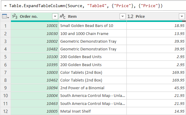
The merged table has loaded from the Power Query Editor into Excel in 8.5 seconds. Unlike formulas, queries do not update automatically. After each change in the source data, you have to update the resulting table manually by clicking the Refresh button on either the Data or Query tab. Our 500,000 rows are refreshed in about 7 seconds. Not bad, but Excel formulas can do better. Considering that setting up a query is far from being a one-click process, this is probably the last method I would use, only if nothing else works.
Performance: loading to Excel 8.5 seconds; refreshing 7.6 seconds
In-depth tutorials:
Extra bonus: Merge Tables Wizard
The users of our Ultimate Suite has one more tool in their Excel toolbox to merge two tables based on a common column. Let's see how it compares with Excel's one.
To run the Merge Tables Wizard, click the Merge Two Tables button on the Ablebits Data tab. And then, just follow the steps of the wizard, and it will walk you through the process.

Well, it took the tool about 3 seconds to complete. Not so bad for half a million records!
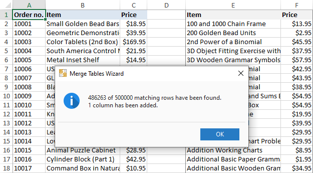
Having a closer look at the message above, you may notice that not all the matches were found. It does not mean, however, that the tool is flawed. It just lets you know that some items (lookup values) do not exist in the lookup table. The VLOOKUP function returns an #N/A error in this case, while the Merge Tables Wizard leaves a cell blank.
Performance: 3.2 seconds
More information: Merge two tables in Excel
Summary and conclusions
If you carefully read though all the examples, then most likely you have already drawn your own conclusions. If you skipped the details, then you can find a quick summary in this comparison table:
| Function | Calculation speed in seconds | |||
|---|---|---|---|---|
| Ranges | Entire columns | Table | Dynamic arrays | |
| VLOOKUP | 6.6 | 14.2 | 2.3 | 1.8 |
| INDEX MATCH | 8.9 | 17.7 | 2.6 | 4.4 |
| OFFSET MATCH | 2.9 | 3.5 | 2.7 | - |
| XLOOKUP | 11.2 | 24.1 | 3.3 | 7.3 |
| Power Query | 8.5 | |||
| Merge Tables | 3.2 | |||
Below, there are a few observations that I made based on the test results. Perhaps, they will be useful for you too.
- Despite all its limitations and drawbacks, VLOOKUP performs quite well, especially with dynamic arrays.
- INDEX MATCH is not as quick as expected. To me, this seems very strange because it processes individual columns, not a table array like VLOOKUP.
- XLOOKUP has many amazing capabilities but is slower than VLOOKUP and INDEX MATCH on huge data sets. Hopefully, Microsoft will improve its performance in the future versions.
- OFFSET MATCH is the fastest in Excel 32-bit. But because of its complex syntax, there a big chance to make a mistake. Also, it does not work with dynamic array, at least I was unable to force it to.
- There is no sense to calculate entire columns unless absolutely necessary. This makes formulas more than twice slower.
- Excel tables rock! To get the most of your Excel, use them wherever possible.
- Dynamic arrays are the future.
Please keep in mind that these observations are based on my tests in dynamic Excel 365, I didn't have an opportunity to test in other versions. If you did, your comments are welcome and will be greatly appreciated!
Practice workbook for download
Fastest VLOOKUP formula in Excel (.xlsx file, 74MB)
 by
by
6 comments
I have a number of situations in which I have two successive VLOOKUPs. As an example, a (partial) UK postcode is resolved into area and county, by looking up the postcode in the first column and returning the second and third columns of the data table. So I may look up a value like "NG32" and get back "Grantham" and "Lincolnshire" in successive columns.
I believe XLOOKUP can return two values in one call; in this situation is one XLOOKUP returning two values faster than a pair of VLOOKUPs?
Also, is an XLOOKUP with its built-in error handling faster than a VLOOKUP wrapped in an IFERROR?
Hi! You can find useful information in these articles: Excel XLOOKUP vs VLOOKUP: differences and advantages and Excel XLOOKUP function with formula examples.
As with your other tutorials, this tutorial is indeed great! What's nice about your works, my dear Svetlana, is that they get to the point in a user-friendly manner. By all means, anyone with a slight background of Excel can directly follow what you are trying to get across. My students are required to refer to your applicable sites when submitting an Excel assignment.
You surely have a way of making things simpler and easier!
Wow. It feels so good to get such a comment from an expert. Thank you so much!
Nice article. I've stop 2 years ago of using vlookups frequently, and start using Index/Match functions instead.Why? Despite in your tests is the fastest , in very large Workbooks with many spreadsheets and on every one is a calculation(s), the use and abuse of vlookup puts the workbook/excel very slow.
Index Match with a lot of data and MANY spreadsheets it's way more light. If you can please confirm.
Cheers
And thank you again for article.
Hi Andre,
Thank you for sharing your experience!
I also gave up Vlookup in favor of Index/Match because of its (Vlookup's) numerous limitations. Our Excel experts say that yes, Vlookup did slow down Excel in very large workbooks, which was especially noticeable in pre-2016 32-bits versions. I say "did" because currently we almost never use Vlookup in practical work, and my test results were a big surprise for us too.
I personally love using Excel tables. However large the table is, any formula calculates in almost no time.