The tutorial shows how to use the VLOOKUP function to copy data from another worksheet or workbook, Vlookup in multiple sheets, and look up dynamically to return values from different sheets into different cells.
When looking up some information in Excel, it's a rare case when all the data is on the same sheet. More often, you will have to search across multiple sheets or even different workbooks. The good news is that Microsoft Excel provides more than one way to do this, and the bad news is that all the ways are a bit more complicated than a standard VLOOKUP formula. But with just a little patience, we will figure them out :)
How to VLOOKUP between two sheets
For starters, let's investigate a simplest case - using VLOOKUP to copy data from another worksheet. It's very similar to a regular VLOOKUP formula that searches on the same worksheet. The difference is that you include the sheet name in the table_array argument to tell your formula in which worksheet the lookup range is located.
The generic formula to VLOOKUP from another sheet is as follows:
As an example, let's pull the sales figures from Jan report to Summary sheet. For this, we define the following arguments:
- Lookup_values are in column A on the Summary sheet, and we refer to the first data cell, which is A2.
- Table_array is the range A2:B6 on the Jan sheet. To refer to it, prefix the range reference with the sheet name followed by the exclamation point: Jan!$A$2:$B$6.
Please pay attention that we lock the range with absolute cell references to prevent it from changing when copying the formula to other cells.
Col_index_num is 2 because we want to copy a value from column B, which is the 2nd column in the table array. - Range_lookup is set to FALSE to look up an exact match.
Putting the arguments together, we get this formula:
=VLOOKUP(A2, Jan!$A$2:$B$6, 2, FALSE)
Drag the formula down the column and you will get this result:
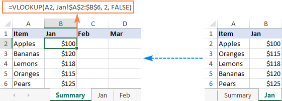
In a similar manner, you can Vlookup data from the Feb and Mar sheets:
=VLOOKUP(A2, Feb!$A$2:$B$6, 2, FALSE)
=VLOOKUP(A2, Mar!$A$2:$B$6, 2, FALSE)
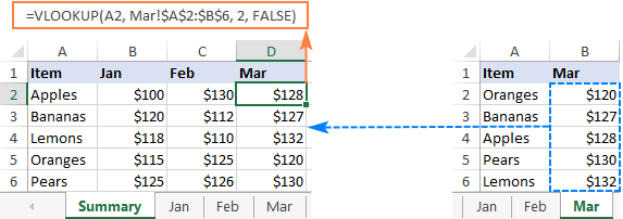
Tips and notes:
- If the sheet name contains spaces or non-alphabetical characters, it must be enclosed in single quotation marks, like 'Jan Sales'!$A$2:$B$6. For more info, please see How to reference another sheet in Excel.
- Instead of typing a sheet name directly in a formula, you can switch to the lookup worksheet and select the range there. Excel will insert a reference with the correct syntax automatically, sparing you the trouble to check the name and troubleshoot.
Vlookup from a different workbook
To VLOOKUP between two workbooks, include the file name in square brackets, followed by the sheet name and the exclamation point.
For example, to search for A2 value in the range A2:B6 on Jan sheet in the Sales_reports.xlsx workbook, use this formula:
=VLOOKUP(A2, [Sales_reports.xlsx]Jan!$A$2:$B$6, 2, FALSE)
For full details, please see VLOOKUP from another workbook in Excel.
Vlookup across multiple sheets with IFERROR
When you need to look up between more than two sheets, the easiest solution is to use VLOOKUP in combination with IFERROR. The idea is to nest several IFERROR functions to check multiple worksheets one by one: if the first VLOOKUP does not find a match on the first sheet, search in the next sheet, and so on.
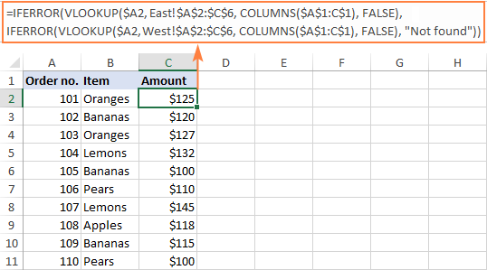
To see how this approach works on real-life data, let's consider the following example. Below is the Summary table that we want to populate with the item names and amounts by looking up the order number in West and East sheets:
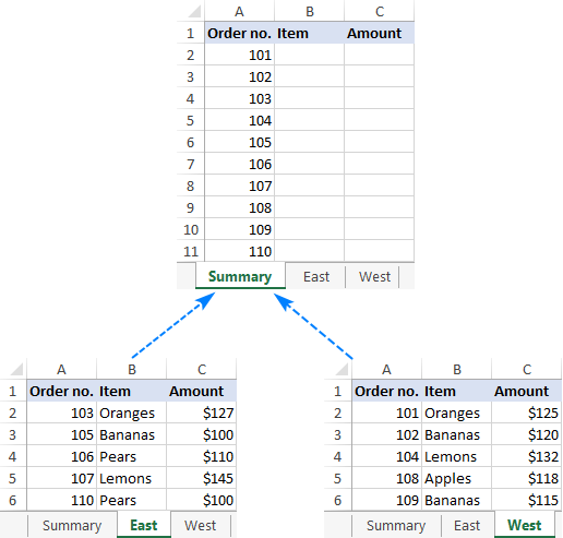
First, we are going to pull the items. For this, we instruct the VLOOKUP formula to search for the order number in A2 on the East sheet and return the value from column B (2nd column in table_array A2:C6). If an exact match is not found, then search in the West sheet. If both Vlookups fail, return "Not found".
=IFERROR(VLOOKUP(A2, East!$A$2:$C$6, 2, FALSE), IFERROR(VLOOKUP(A2, West!$A$2:$C$6, 2, FALSE), "Not found"))
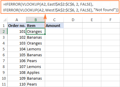
To return the amount, simply change the column index number to 3:
=IFERROR(VLOOKUP(A2, East!$A$2:$C$6, 3, FALSE), IFERROR(VLOOKUP(A2, West!$A$2:$C$6, 3, FALSE), "Not found"))
Tip. If needed, you can specify different table arrays for different VLOOKUP functions. In this example, both lookup sheets have the same number of rows (A2:C6), but your worksheets may be different in size.
Vlookup in multiple workbooks
To Vlookup between two or more workbooks, enclose the workbook name in square brackets and put it before the sheet name. For example, here's how you can Vlookup in two different files (Book1 and Book2) with a single formula:
=IFERROR(VLOOKUP(A2, [Book1.xlsx]East!$A$2:$C$6, 2, FALSE), IFERROR(VLOOKUP(A2, [Book2.xlsx]West!$A$2:$C$6, 2, FALSE),"Not found"))
Make column index number dynamic to Vlookup multiple columns
In situation when you need to return data from several columns, making col_index_num dynamic could save you some time. There are a couple of adjustments to be made:
- For the col_index_num argument, use the COLUMNS function that returns the number of columns in a specified array: COLUMNS($A$1:B$1). (The row coordinate does not really matter, it can be just any row.)
- In the lookup_value argument, lock the column reference with the $ sign ($A2), so it remains fixed when copying the formula to other columns.
As the result, you get a kind of dynamic formula that extracts matching values from different columns, depending on which column the formula is copied to:
=IFERROR(VLOOKUP($A2, East!$A$2:$C$6, COLUMNS($A$1:B$1), FALSE), IFERROR(VLOOKUP($A2, West!$A$2:$C$6, COLUMNS($A$1:B$1), FALSE), "Not found"))
When entered in column B, COLUMNS($A$1:B$1) evaluates to 2 telling VLOOKUP to return a value from the 2nd column in the table array.
When copied to column C (i.e. you've dragged the formula from B2 to C2), B$1 changes to C$1 because the column reference is relative. Consequently, COLUMNS($A$1:C$1) evaluates to 3 forcing VLOOKUP to return a value from the 3rd column.
This formula works great for 2 - 3 lookup sheets. If you have more, repetitive IFERRORs become too cumbersome. The next example demonstrates a bit more complicated but a lot more elegant approach.
Vlookup multiple sheets with INDIRECT
One more way to Vlookup between multiple sheets in Excel is to use a combination of VLOOKUP and INDIRECT functions. This method requires a little preparation, but in the end, you will have a more compact formula to Vlookup in any number of spreadsheets.
A generic formula to Vlookup across sheets is as follows:
Where:
- Lookup_sheets - a named range consisting of the lookup sheet names.
- Lookup_value - the value to search for.
- Lookup_range - the column range in the lookup sheets where to search for the lookup value.
- Table_array - the data range in the lookup sheets.
- Col_index_num - the number of the column in the table array from which to return a value.
For the formula to work correctly, please bear in mind the following caveats:
- It's an array formula, which must be completed by pressing Ctrl + Shift + Enter keys together.
- All the sheets must have the same order of columns.
- As we use one table array for all lookup sheets, specify the largest range if your sheets have different numbers of rows.
How to use the formula to Vlookup across sheets
To Vlookup multiple sheets at a time, carry out these steps:
- Write down all the lookup sheet names somewhere in your workbook and name that range (Lookup_sheets in our case).

- Adjust the generic formula for your data. In this example, we'll be:
- searching for A2 value (lookup_value)
- in the range A2:A6 (lookup_range) in four worksheets (East, North, South and West), and
- pull matching values from column B, which is column 2 (col_index_num) in the data range A2:C6 (table_array).
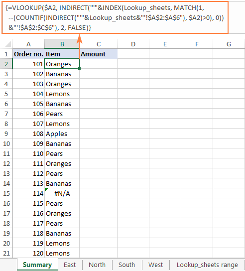
With the above arguments, the formula takes this shape:
=VLOOKUP($A2, INDIRECT("'"&INDEX(Lookup_sheets, MATCH(1, --(COUNTIF(INDIRECT("'"& Lookup_sheets&"'!$A$2:$A$6"), $A2)>0), 0)) &"'!$A$2:$C$6"), 2, FALSE)Please notice that we lock both ranges ($A$2:$A$6 and $A$2:$C$6) with absolute cell references.
- Enter the formula in the topmost cell (B2 in this example) and press Ctrl + Shift + Enter to complete it.
- Double click or drag the fill handle to copy the formula down the column.
As the result, we've got the formula to look up the order number in 4 sheets and retrieve the corresponding item. If a specific order number is not found, a #N/A error is displayed like in row 14:
To return the amount, simply replace 2 with 3 in the col_index_num argument as amounts are in the 3rd column of the table array:
=VLOOKUP($A2, INDIRECT("'"&INDEX(Lookup_sheets, MATCH(1, --(COUNTIF(INDIRECT("'" & Lookup_sheets & "'!$A$2:$A$6"), $A2)>0), 0)) & "'!$A$2:$C$6"), 3, FALSE)
If you'd like to replace the standard #N/A error notation with your own text, wrap the formula into the IFNA function:
=IFNA(VLOOKUP($A2, INDIRECT("'"&INDEX(Lookup_sheets, MATCH(1, --(COUNTIF(INDIRECT("'" & Lookup_sheets & "'!$A$2:$A$6"), $A2)>0), 0)) & "'!$A$2:$C$6"), 3, FALSE), "Not found")

Vlookup multiple sheets between workbooks
This generic formula (or its any variation) can also be used to Vlookup multiple sheets in a different workbook. For this, concatenate the workbook name inside INDIRECT like shown in the below formula:
=IFNA(VLOOKUP($A2, INDIRECT("'[Book1.xlsx]" & INDEX(Lookup_sheets, MATCH(1, --(COUNTIF(INDIRECT("'[Book1.xlsx]" & Lookup_sheets & "'!$A$2:$A$6"), $A2)>0), 0)) & "'!$A$2:$C$6"), 2, FALSE), "Not found")
Vlookup between sheets and return multiple columns
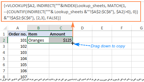
If you want to pull data from several columns, a multi-cell array formula can do that in one go. To create such a formula, supply an array constant for the col_index_num argument.
In this example, we wish to return the item names (column B) and amounts (column C), which are the 2nd and 3rd columns in the table array, respectively. So, the required array is {2,3}.
=VLOOKUP($A2, INDIRECT("'"&INDEX(Lookup_sheets, MATCH(1, --(COUNTIF(INDIRECT("'"& Lookup_sheets &"'!$A$2:$C$6"), $A2)>0), 0)) &"'!$A$2:$C$6"), {2,3}, FALSE)
To correctly enter the formula in multiple cells, this is what you need to do:
- In the first row, select all the cells to be populated (B2:C2 in our example).
- Type the formula and press Ctrl + Shift + Enter. This enters the same formula in the selected cells, which will return a different value in each column.
- Drag down the formula to the remaining rows.
How this formula works
To better understand the logic, let's break down this basic formula to the individual functions:
=VLOOKUP($A2, INDIRECT("'"&INDEX(Lookup_sheets, MATCH(1, --(COUNTIF(INDIRECT("'"& Lookup_sheets&"'!$A$2:$A$6"), $A2)>0), 0)) &"'!$A$2:$C$6"), 2, FALSE)
Working from the inside out, here's what the formula does:
COUNTIF and INDIRECT
In a nutshell, INDIRECT builds the references for all lookup sheets, and COUNTIF counts the occurrences of the lookup value (A2) in each sheet:
--(COUNTIF( INDIRECT("'"&Lookup_sheets&"'!$A$2:$A$6"), $A2)>0)
In more detail:
First, you concatenate the range name (Lookup_sheets) and the range reference ($A$2:$A$6), adding apostrophes and the exclamation point in the right places to make an external reference, and feed the resulting text string to the INDIRECT function to dynamically refer to the lookup sheets:
INDIRECT({"'East'!$A$2:$A$6"; "'South'!$A$2:$A$6"; "'North'!$A$2:$A$6"; "'West'!$A$2:$A$6"})
COUNTIF checks each cell in the range A2:A6 on each lookup sheet against the value in A2 on the main sheet and returns the count of matches for each sheet. In our dataset, the order number in A2 (101) is found in the West sheet, which is 4th in the named range, so COUNTIF returns this array:
{0;0;0;1}
Next, you compare each element of the above array with 0:
--({0; 0; 0; 1}>0)
This yields an array of TRUE (greater than 0) and FALSE (equal to 0) values, which you coerce to 1's and 0's by using a double unary (--), and get the following array as the result:
{0; 0; 0; 1}
This operation is an extra precaution to handle a situation when a lookup sheet contains several occurrences of the lookup value, in which case COUNTIF would return a count greater than 1, while we want only 1's and 0's in the final array (in a moment, you will understand why).
After all these transformations, our formula looks as follows:
VLOOKUP($A2, INDIRECT("'"&INDEX(Lookup_sheets, MATCH(1, {0;0;0;1}, 0)) &"'!$A$2:$C$6"), 2, FALSE)
INDEX and MATCH
At this point, a classic INDEX MATCH combination steps in:
INDEX(Lookup_sheets, MATCH(1, {0;0;0;1}, 0))
The MATCH function configured for exact match (0 in the last argument) looks for the value 1 in the array {0;0;0;1} and returns its position, which is 4:
INDEX(Lookup_sheets, 4)
The INDEX function uses the number returned by MATCH as the row number argument (row_num), and returns the 4th value in the named range Lookup_sheets, which is West.
So, the formula further reduces to:
VLOOKUP($A2, INDIRECT("'"&"West"&"'!$A$2:$C$6"), 2, FALSE)
VLOOKUP and INDIRECT
The INDIRECT function processes the text string inside it:
INDIRECT("'"&"West"&"'!$A$2:$C$6")
And converts it into a reference that goes to the table_array argument of VLOOKUP:
VLOOKUP($A2, 'West'!$A$2:$C$6, 2, FALSE)
Finally, this very standard VLOOKUP formula searches for the A2 value in the first column of the range A2:C6 on the West sheet and returns a match from the 2nd column. That's it!
Dynamic VLOOKUP to return data from multiple sheets into different cells
First off, let's define what exactly the word "dynamic" means in this context and how this formula is going to be different from the previous ones.
In case you have large chunks of data in the same format that are split over multiple spreadsheets, you may want to extract information from different sheets into different cells. The image below illustrates the concept:
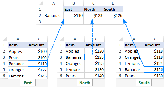
Unlike the previous formulas that retrieved a value from a specific sheet based on a unique identifier, this time we are looking to extract values from several sheets at a time.
There are two different solutions for this task. In both cases, you need to do a little preparatory work and create named ranges for data cells in each lookup sheet. For this example, we defined the following ranges:
- East_Sales - A2:B6 on the East sheet
- North_Sales - A2:B6 on the North sheet
- South_Sales - A2:B6 on the South sheet
- West_Sales - A2:B6 on the West sheet
VLOOKUP and nested IFs
If you have a reasonable number of sheets to look up, you can use nested IF functions to select the sheet based on the keywords in the predefined cells (cells B1 through D1 in our case).
With the lookup value in A2, the formula is follows:
=VLOOKUP($A2, IF(B$1="east", East_Sales, IF(B$1="north", North_Sales, IF(B$1="south", South_Sales, IF(B$1="west", West_Sales)))), 2, FALSE)
Translated into English, the IF part reads:
If B1 is East, look in the range named East_Sales; if B1 is North, look in the range named North_Sales; if B1 is South, look in the range named South_Sales; and if B1 is West, look in the range named West_Sales.
The range returned by IF goes to table_array of VLOOKUP, which pulls a matching value from the 2nd column on the corresponding sheet.
The clever use of mixed references for the lookup value ($A2 - absolute column and relative row) and the logical test of IF (B$1 - relative column and absolute row) allows copying the formula to other cells without any changes - Excel adjusts the references automatically based on the relative position of a row and column.
So, we enter the formula in B2, copy it right and down to as many columns and rows as needed, and get the following result:

INDIRECT VLOOKUP
When working with many sheets, multiple nested levels could make the formula too lengthy and difficult to read. A far better way is to create a dynamic vlookup range with the help of INDIRECT:
=VLOOKUP($A2, INDIRECT(B$1&"_Sales"), 2, FALSE)
Here, we concatenate the reference to the cell that contains a unique part of the named range (B1) and the common part (_Sales). This produces a text string like "East_Sales", which INDIRECT converts to the range name understandable by Excel.
As the result, you get a compact formula that works beautifully on any number of sheets:

That's how to Vlookup between sheets and files in Excel. I thank you for reading and hope to see you on our blog next week!
Practice workbook for download
Vlookup multiple sheets examples (.xlsx file)
 by
by
194 comments
Hi
I have entered the following formula and getting error message. "Formula is missing an opening or closing parenthesis"
=IF([@[Profit Center]]="300","ABC",IF([@[Profit Center]]="400","DEF",IF([@[Profit Center]]="410","GHI",IF([@[Profit Center]]="420","XYZ","").
could you please advise this error. Thank you
Hi! To write down the formula correctly, study these instructions carefully: Structured reference in Excel tables.
Your formulas are missing the name of the Excel table.
Thanks, this helped me add dynamic sheet names into my vlookup
Hi
I have tried the Vlookup across multiple sheets with INDIRECT, but it does not work. my
Lookupsheets - multiple worksheets
lookup value - A3112
lookup Range = AD:AD ( column in lookupsheets)
Table array = A:AD (data range in the lookupsheets)
This is the formula I am using
=VLOOKUP(A3112,INDIRECT("'"&INDEX(Lookupsheets,MATCH(1,--(COUNTIF(INDIRECT("'"&Lookupsheets&AD:AD),A3112)>0),0))&A:AD),30,FALSE)
Hi! I can't understand and test your formula because I don't know what data it uses. What does "Lookupsheets - multiple worksheets" mean? To learn how to do a multi-sheet search, read the article above carefully.
To find out the correct way to create a reference to a worksheet using the INDIRECT function, look here: Creating an Excel dynamic reference to another sheet.
Hi! I m in great difficulty. I am using Excel 2016 and want to fill information in Book1 Sheet1, ColumnB2 with reference to the value in Book1, sheet1, column A2(lookup_value), the information is to be fetched / vlookedup from Book2, (sheet1/sheet2/sheet3/..../sheet11) {any one of them}, columnB2. hope you understand. waiting for reply.
Hi! If I understand your task correctly, this guide may be helpful: How to VLOOKUP across multiple sheets in Excel with examples. Since your explanations are not very clear, it's hard to suggest a formula.
Yes. I tried my level best to elaborate & simplify the requirement, anyhow, i want to fetch data from Book2 which has 11 sheets, in Book1. Book1 & Book2 obviously are different excel files.
Hi! Use external references to other workbooks in your VLOOKUP formulas, as described in this article: How to Vlookup from another workbook in Excel.
Hello
I hope you can help me.
In sheet A, column L, I have a Narrative from timesheets e.g. CRM Is 964016 - Project x - TS14nnnnn
In sheet B, column A, I have a list of the CRM IDs that relate to that project ID
I want Excel to look up sheet B, column A to see if sheet A column L has the same number in amongst the text and put either the number or n/a in sheet A, column S.
Can this be done?
Hello! If I understand you correctly, you want to determine the partial match between the text in column A and the text in column L. Based on the information given, the formula could be as follows:
=INDEX(B!$A$1:$A$10,MATCH(TRUE,ISNUMBER(SEARCH(" "&B!$A$1:$A$10&" ",A!L1)),0))
For more information, please read: How to find substring in Excel
Use INDEX MATCH to get the value that matches the partial match found.
Alexander, thank you so much, I've been working on this for weeks. I just had to tweek the actual names of the tabs and voila!
Hi,
Thank you for your helpful lessons. I tried your formula to look up in multiple sheets name sheet1, sheet2, sheet3
LOOKUP(lookup_value, INDIRECT("'"&INDEX(Lookup_sheets, MATCH(1, --(COUNTIF(INDIRECT("'" & Lookup_sheets & "'!lookup_range"), lookup_value)>0), 0)) & "'!table_array"), col_index_num, FALSE)
my lookup sheet range:
Sheet1
Sheet2
Sheet3
but it only gets the result from sheet1 only, if I change my lookup sheet range to:
Sheet3
Sheet1
Sheet2
the result of sheet3 will be shown
I don't know what's wrong...
Can you please help?
Thanks a lot
Hi! I can't check a formula that contains unique references to your data, which I don't have.
Note whether you are correctly using named ranges: Lookup_sheets, lookup_range, lookup_value, table_array, col_index_num.
Read more: Excel names and named ranges: how to define and use in formulas.
Hi,
I have 2 sheets within a single workbook. My first sheet has students' ID numbers, students' test scores, teachers, etc. My second sheet has students' ID numbers, students' teachers and the class periods that students have the teachers. I am trying to pull the class periods from sheet 2 and return it to sheet one (where student test scores are located) using the students' ID numbers that are in both. The formula that I am using is =VLOOKUP(B2,'Class Rosters'!A:E,3,false). I am getting #N/A error message. What am I doing wrong?
Hi! I can't check a formula that contains unique references to your data, which I don't have.
Here is the article that may be helpful to you: Fixing #N/A error in VLOOKUP.
Hi Guys. I need some help please.
I used your formula in my excel file: =IFNA(VLOOKUP($A2, INDIRECT("'"&INDEX(Lookup_sheets, MATCH(1, --(COUNTIF(INDIRECT("'" & Lookup_sheets & "'!$A$2:$A$6"), $A2)>0), 0)) & "'!$A$2:$C$6"), 3, FALSE), "Not found") and worked brilliantly, until it didn't :)).
I have an Excel file with multiple tabs in which I am trying to keep track of my timesheets per project/per week. First is the summary and the rest are week 1 (W01) till week 52 (W52) .
Every week sheet has a column with project code, another column with the project name and then weekdays column indicating the hrs worked on the specific project that week. Some weeks have on project, some weeks have multiple projects. There are projects that spread over multiple weeks as well as one week only.
While I am trying to build up a summary tab with all the info in one place, I found your formula, pasted above, and used it in my summary tab and seems to work only for the first 6 returned matched values and after it doesn't return the match-up value.
I try to recreate bellow the layout of my summary tab and use some generic term for the sake of simplicity.
Nr.Crt. Project Code Project Name
1 20021 Project x
2 20022 Project a
3 20033 Project y
4 20011 Project z
5 11000 Project c
6 212121 Project v
7 32321 empty or "not found"
8 445667 empty or "not found"
Can you please advise why this happens?!.
Thanks a lot in advance.
Regards,
Peter
Hi! If you look at it carefully, the formula works for the first six rows because it uses the range $A$2:$A$6. Use the range you need.
Thanks a lot Alexander. It was indeed the range. Having it adjusted, it works fine
So basically I want to fill in the Project Name column with the corresponding names to the project code found throughout the week sheet tabs and compiled in the Project Code column.
Good afternoon everyone,
I have a sheet that contains multiple columns of information (date, then name, course, lab #, lab completed? Yes/No, etc., that are selected from dropdown menus). The line information is manually entered each time a student checks out an item to complete their lab.
If Yes is selected from the lab completed column, I would like the date associated with that name, course, lab # to be auto-populated into the correct course sheet tab and associated lab (there are nine different course sheet tabs and anywhere from 10 - 15 different lab # columns in each sheet).
I'm not sure where to start with this one. Any help is appreciated.
Cheers
Good evening Alexander,
I've tried a variety of formulas, and I can use the following formula to pull a date from my CheckOut sheet, and into my Lab sheet:
=INDEX(CheckOut!B:B,MATCH($A3,CheckOut!$A:$A,0),0)
CheckOut!B:B refers to column B, dates in the CheckOut sheet, and CheckOut!$A:$A refers to column A, student names in the CheckOut sheet. $A3 refers to column A, student names in the Lab sheet.
However, I need to expand the formula to verify that a specific Lab #, column D in the CheckOut sheet, is selected as "YES" from column E in the CheckOut sheet before pulling the date from the CheckOut sheet into the specific Lab # column in the Lab sheet.
Still trying to solve this fun puzzle :)
Cheers
Hi! If I understand your task correctly, this article may be helpful: Excel INDEX MATCH with multiple criteria - formula examples.
Good evening Alexander,
Brilliant article recommend. I was able to use the multiple match, and modify the formula to meet my multi tab needs with multiple match criteria. Thank you again!
Cheers
Hi! If I understand your task correctly, you can get all of a course or lab's records from a common dataset using a pivot table or by using the FILTER function. I recommend reading these guides: How to make and use Pivot Table in Excel and Excel FILTER function - dynamic filtering with formulas.
This is driving me nuts, so hopefully you can help. I have a spreadsheet with seven worksheets. The first sheet has my data to lookup, the other six sheets have data about some of the values I need to lookup. What I want to do is look for the data in Sheet1 A2 and return the sheet name it finds the lookup value in first. In other words, if sheet1 A2 is "test", I want to look for test in the other sheets, and if the first place it finds test is in Sheet4, I need to return the name of that tab (Sheet4). I have a formula to return the name of the tab in column C of each sheet ( =RIGHT(CELL("filename",A2),LEN(CELL("filename",A2))-FIND("]",CELL("filename",A2),1)) ) which works great if I'm only looking for the name of one sheet. When I copy that formula to each sheet's column C, it gives me the name of the sheet the formula was last run on across all of the sheets, which I thought was kind of weird. I tried the "VLOOKUP across multiple sheets with IFERROR" formula to pull this sheet name from column C, which is how I discovered that it returns the name of the sheet the formula was last run on. Any idea how I can do this?
Hi! To return the name of the worksheet on which the value from cell A2 is found in column A, try this formula:
=IFNA(INDEX(Lookup_sheets,MATCH(1,--(COUNTIF(INDIRECT("'"&Lookup_sheets&"'!$A$2:$A$20"),$A2)>0),0)),"Not found")
Lookup_sheets - named range with the names of all worksheets
Grade 1 2 3 4 5 6 7 8 9 10 11 12 13 14 15
Step 1 $24,464 $27,508 $30,015 $33,693 $37,696 $42,022 $46,696 $51,713 $57,118 $62,898 $69,107 $82,830 $98,496 $116,393 $136,908
Step 2 $25,285 $28,163 $31,016 $34,816 $38,953 $43,422 $48,252 $53,437 $59,021 $64,995 $71,410 $85,591 $101,779 $120,272 $141,472
Step 3 $26,097 $29,074 $32,017 $35,939 $40,210 $44,822 $49,808 $55,162 $60,925 $67,092 $73,713 $88,352 $105,062 $124,152 $146,035
Step 4 $26,908 $29,844 $33,017 $37,062 $41,467 $46,223 $51,365 $56,886 $62,828 $69,189 $76,016 $91,113 $108,345 $128,031 $150,598
Step 5 $27,720 $30,180 $34,018 $38,185 $42,724 $47,623 $52,921 $58,610 $64,732 $71,286 $78,319 $93,875 $111,628 $131,911 $155,162
Step 6 $28,195 $31,068 $35,019 $39,308 $43,981 $49,023 $54,478 $60,334 $66,636 $73,383 $80,623 $96,636 $114,911 $135,790 $159,725
Step 7 $29,000 $31,956 $36,019 $40,431 $45,238 $50,424 $56,034 $62,058 $68,539 $75,480 $82,926 $99,397 $118,194 $139,670 $164,288
Hello there, I am working on salary and I have been asked to look for the salary pay showing the grade and step. An employee earns yearly $60,950, I need to search, what is this employee grade and step. Please advise on how to vlookup or other command that is best for this task. Thank you.
Hi! If I understand correctly, you want to find the closest number to the employee's earns and determine which row and column it is in. Here is an example of the formulas:
Row number -
=MIN(IF(MIN(ABS(A2:E5-G3))=ABS(A2:E5-G3),ROW(F2:F5)))
Column number -
=MIN(IF(MIN(ABS(A2:E5-G3))=ABS(A2:E5-G3),COLUMN(A2:E2)))
G3 - employee earns
Good Morning
I need help figuring out how to pull multiple instances of an activity from a range of cells on one tab and list all of those activities into a single cell on a second tab. We have a Work Plan with activities that we are required to complete during the year. We also have an Activities Tracker that we use to log our daily activities. I need to pull the information from the Activities Tracker and list it in a single cell on the Work Plan page. For example, the Work Plan requires us to complete Planning Meetings. On the Activities Tracker there may be 7 or 10 or more instances of Planning Meetings. How would I pull all of the Planning Meetings from the range of cells on the Activity Tracker Tab and list them into the single Planning Meeting cell on the Work Plan Tab? The formula I have tried will only list the first instance of the activities but will not pull subsequent instances of an activity into the Work Plan Tab.
Thanks in advance!
Hi! Unfortunately, without seeing your data it is difficult to give you any advice.
I want to extract two columns from first sheet to 2nd sheet.
Data range is D4:I50
Columns: Control # Party Name Start Date End Date Status Category
-------------------------------------------------------------------------------------------------------------------------
Date: Active Commercial
Required rows are on the basis of last two columns value "Active" and "Commercial".
Please guide.
Hello! You can use the FILTER function to extract part of the data from the range based on the criterion. You can find the examples and detailed instructions here: Excel FILTER function - dynamic filtering with formulas. Hope this is what you need.
Hi there Alexander,
I am trying to use the following formula: =VLOOKUP($A2, INDIRECT("'"&INDEX(Lookup_sheets, MATCH(1, --(COUNTIF(INDIRECT("'"& Lookup_sheets&"'!$A$2:$A$6"), $A2)>0), 0)) &"'!$A$2:$C$6"), 2, FALSE) to get data from different sheets into 1 sheet.
On my sheet where I am trying to aggregate all data, the different tabs are layed out below each other (so all tab names are in 1 column). When I try to copy the formula down, it gives the same number from only the very first tab and not a 'rolling' basis, as in, I don't receive the numbers from the other tabs. This means there is 1 small part missing in my formula where I don't get the other values from the different tabs in one column when dragging down below.
Could you please help me with this?
Best,
Tim
Hello! This formula works for me, but I cannot test it with your data. Try using the example file referenced at the end of this article.
Hello Alex,
In an excel workbook , I have 45 worksheets/ tabs. The master data resides in the first sheet with all the item data while the other sheets represent each item category. The data structure is the same across the 44 sheets and is an extract of the data from the master sheet. I keep adding additional columns in the master sheet as and when I receive data from the source; I add these columns on each of the 44 sheets too. My question is how do I add these new columns together with the values across the 44 sheets in one go!! Item Code is the common reference value between the master sheet and the other 44 sheets.
Hello! You can only add data to a master sheet and extract the desired data for each item from the master sheet using the pivot table or the FILTER function. I hope it’ll be helpful. If something is still unclear, please feel free to ask.
Hello,
I have this data in one sheet. Need to Order: 10 30 20 (in one rows, cell number D40, E40, F40).
I want to insert this data in another sheet called 'Product List' in 'Order' column (in columns, cell number E3, E4, E5).
Can you please help me.
Hi! Here is the article that may be helpful to you: Excel reference to another sheet or workbook (external reference).
I am trying to fetch data from each sheet of a different workbook (ABC.xlsx). Sheet names are changing as per Date. Example:
05-24-2023
05-25-2023
05-26-2023
Currently I am using formula:
=VLOOKUP(B2,[ABC.xlsx]05-24-2023!$E$2:$F$7,2,FALSE)
Please let me know how I can make the sheet name dynamic (vary as per date. As per above example).
Hi! Try to use the recommendations described in this article: INDIRECT formula to dynamically refer to another worksheet. I hope my advice will help you solve your task.
Sir,
Can you give me syntax for searching an item through multiple sheets by using index match
Thanks
Hi! Just replace VLOOKUP with INDEX MATCH in the sample formulas you see above. If there is a specific question, you can ask it in the comments.
I have all the names of the sheets written in one column of another sheet
VLOOKUP and INDEX MATCH can search in only one data range.
Sir, thanks for the quick reply.
my formula is
=IFERROR(INDEX(INDIRECT("'"&A2&"'!$C$5:$P"),MATCH($F$13,INDIRECT("'"&A2&"'!$M$5:$M"),0),11),"")
here I want to search from A2 to A12 dynamically and find the sheet name where F13 matches
Hi! Note that $C$5:$P and $M$5:$M - incorrect references. Read more: Excel cell reference: how to make and use.
=IFERROR(INDEX(INDIRECT("'"&A2&"'!$A$5:$P"),MATCH($F$13,INDIRECT("'"&A2&"'!$M$5:$M"),0),13),"")
only one column (ie M) to be searched in all the sheets
Hi,
I have created a spreadsheet for an event to record results.
I have a names tab which collates rider and horse and concatenates it to create a unique combo. I then have an event tab which hyperlinks to individual tab for each event and records 1st, 2nd, 3rd placing which is then converted to points ie. 1st = 5 points, 2nd = 3 points in a second column. Ihave each results tab set up identical so it is consistent across the board.
I now need to set up a summary sheet to calculate all points per rider and horse combination. I have used a vlookup to this effect - =vlookup(a2,tab1 a:f, 6,false)+vlookup(a2,tab2 a:f,6,false)+……
The first vlookup works, but as soon as I add the second (or more) it fails. Because I may have only calculated points in the first event and not the second. So I get an #refs error.
Is this the best way to total the points? Or is there a better formula?
Any suggestions would be appreciated.
Sir I have 2 work sheets i.e 1 updated demand of 1500 assessments yearwise in commons.2 with the help of v lookup formula i created a receipt indicating year wise payments referring assessment as the base.my problem is if an assessed is not interested to pay entire due amount how ican stop the cell values for which assessed is not paying for. Secondly how I can make up dated demand zero or make demand zero for the years for which assessed paid for.